… or how I stopped trusting standardized coefficients.
Say you want to know how perceived importance of job security is related to feelings of job satisfaction. Let’s also say that you suspect that this relationship might differ between Gen-X-ers and millennials with their MTV and their hip-hop. So you conduct a survey, asking 100 Gen-X-ers and 100 millennials to rank how important they think job security is when job searching and their current job satisfaction. You then plug your data into a 2-step hierarchical regression to test the moderating effect of Generation on the effect of Job Security in your favorite stats program (If you’re a Gen-X-er, SPSS. If you’re a millennial, or a reasonable human being, R). You find:
| (Intercept) |
4.400 |
0.393 |
11.203 |
<0.001 |
| Group [Millennial] |
0.575 |
0.245 |
2.343 |
0.020 |
| Job Security |
0.450 |
0.046 |
9.717 |
<0.001 |
| (Intercept) |
3.20 |
0.527 |
6.076 |
<0.001 |
| Group [Millennial] |
2.45 |
0.613 |
3.994 |
<0.001 |
| Job Security |
0.60 |
0.064 |
9.391 |
<0.001 |
| Group [Millennial] * Job Security |
-0.30 |
0.090 |
-3.320 |
0.001 |
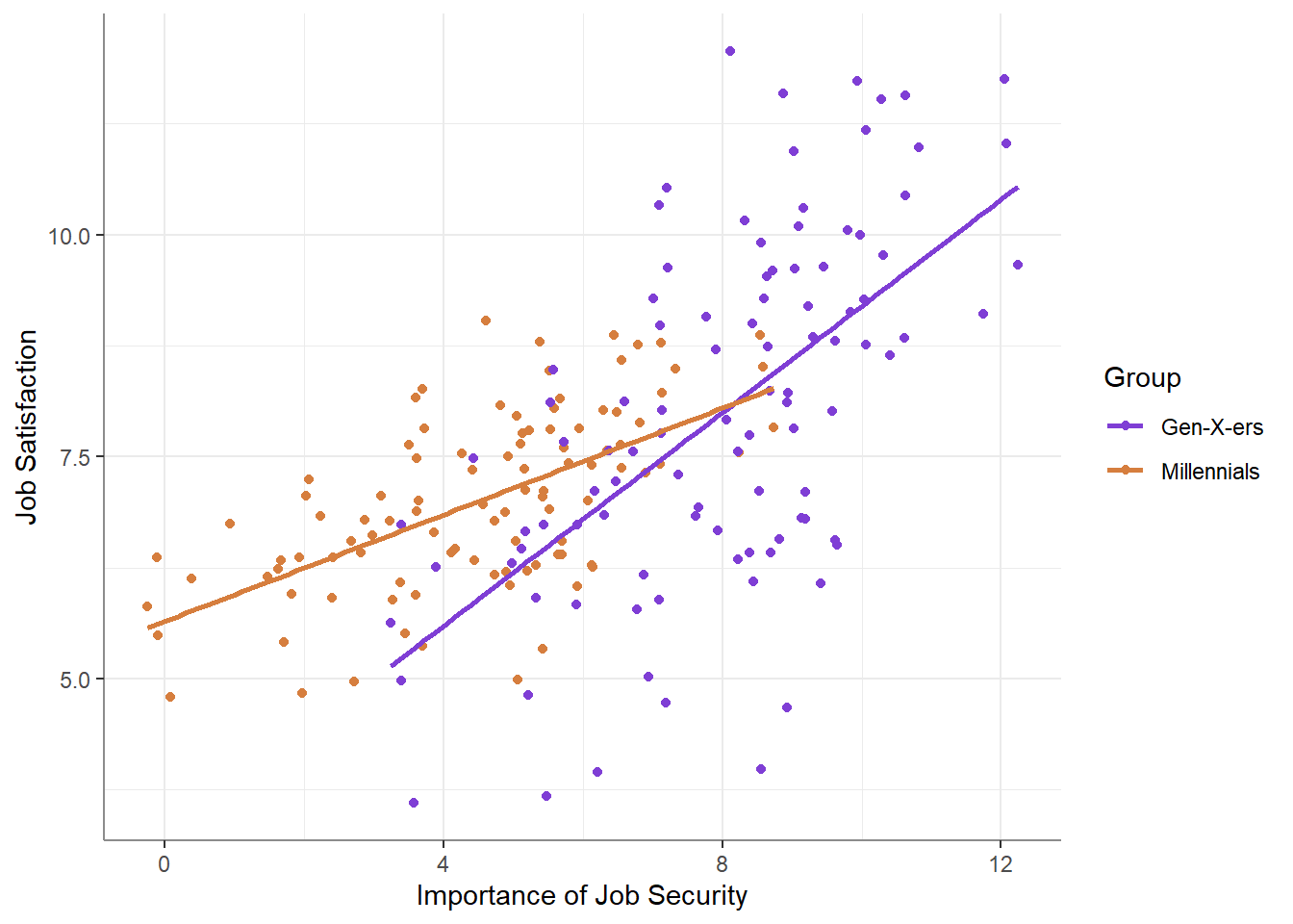
“Very interesting”, you think to yourself. But before drafting your Science submission, you decide to plot your data, just to make sure this trend isn’t somehow driven by outliers, and you find that it is not!
`geom_smooth()` using formula = 'y ~ x'
“This is great!” you confidently think to yourself, “The relationship between the perceived importance of job security and reported job satisfaction is weaker among millennials!”. But how much weaker? You extract the simple slopes for both groups:
| Gen-X-ers |
0.6 |
0.064 |
196 |
9.391 |
<0.001 |
| Millennials |
0.3 |
0.064 |
196 |
4.696 |
<0.001 |
A slope of 0.6 for Gen-X-ers and of 0.3 for Millennials. You find it hard to interpret these slopes, so you do the next reasonable thing: you decide to standardize job security importance and job satisfaction.
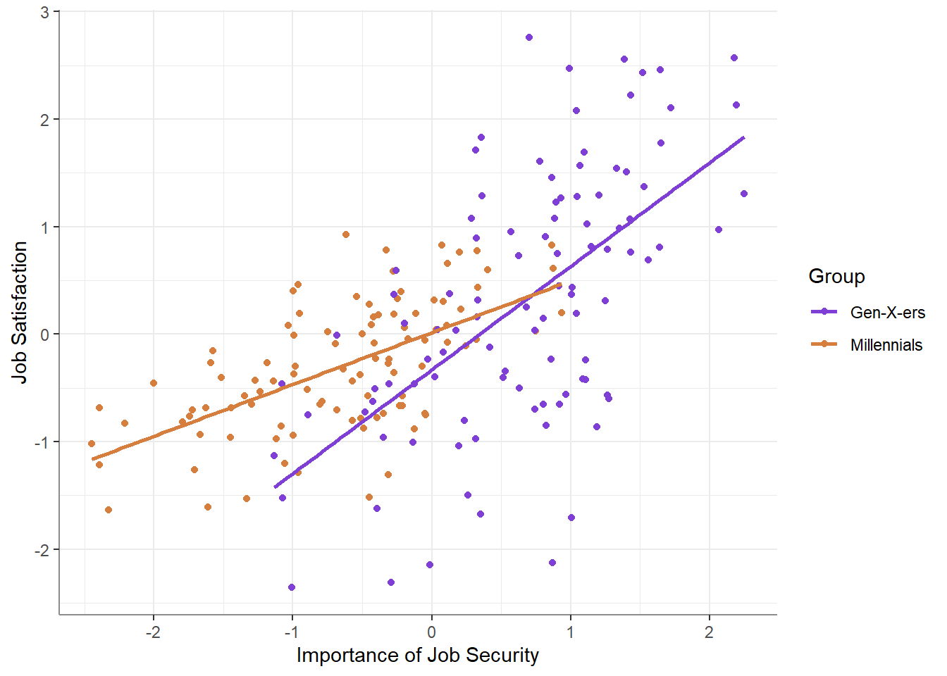
Just to make sure nothing funny happened, you plot your data again:
`geom_smooth()` using formula = 'y ~ x'
As expected - your data is now scaled and centered! You compute the simple standardized slopes and find that:
| Gen-X-ers |
0.963 |
0.103 |
196 |
9.391 |
<0.001 |
| Millennials |
0.482 |
0.103 |
196 |
4.696 |
<0.001 |
“Amazing,” you exclaim to yourself,” the relationship between importance of job security and job satisfaction is nearly perfect among Gen-X-ers, and is half as strong among millennials!” You open MS Word and start typing away…
Something’s not right.
But wait - looking at the plot above, it is clear that the correlation among Gen-X-ers is far from perfect! How is this possible? What’s really going on here?
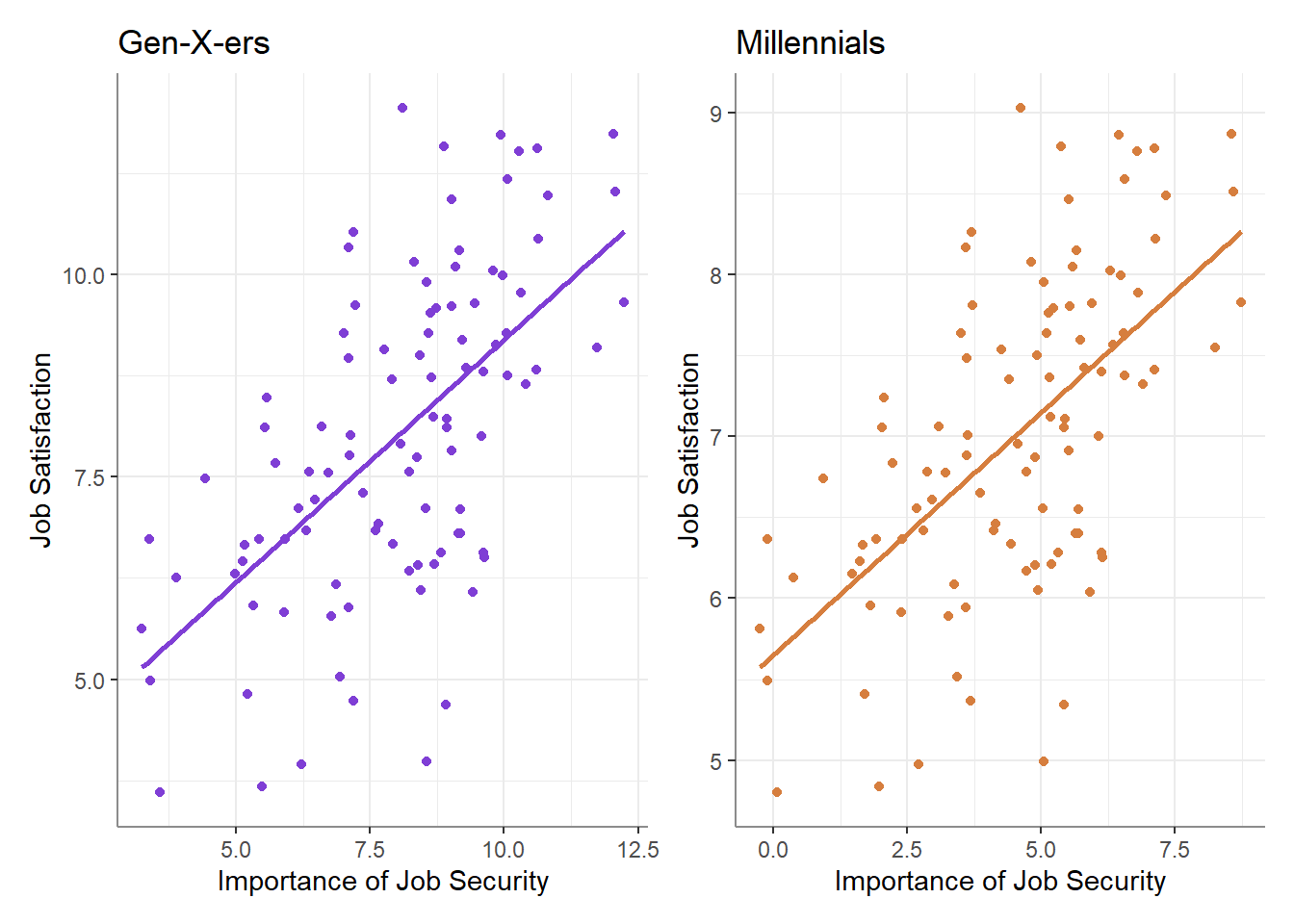
The short answer is that that the strength of the association (i.e., the correlation) does not equal the strength of the effect (i.e., the slope). Plotting the relationship for each group separately will shed some light on what’s actually going on:
As is now apparent, the strength of the correlation is equal between the groups - if we were to calculate the correlation between within each group, we would find that they are both exactly \(r=0.6\) (in fact, you can see that I made the scatter of points literally identical between the groups), with the only difference between the groups being the difference in scale (and center) of the two variables.
Why does this happen?
The slope, even the standardized slope, only measures the expected change in our outcome variable (e.g., Job Satisfaction) as a function of change in a predictor’s values (e.g., Perceived Importance of Job Security). If we’ve standardized our data, the only thing we’ve changed is that the slope now represents the expected change in an outcome’s standardized values as a function of a change in the predictor’s standardized values.
But why does this not yield what we expect? If in a simple regression analysis the standardized slope is the correlation (i.e., the strength of the relationship), why is that not the case here when measuring simple standardized slopes?
The reason is that when we standardize a variable, we standardize it across any other variables that might interact with it, while our question regards the standardized change in \(Y\) as a function of \(X\) within different levels of a moderator variable.
What can we do?
The first thing we should do is understand what we are estimating and testing when fitting a moderation model: we are testing whether the size of variable \(X\)’s effect on variable \(Y\) is different within different levels of some other \(M\) variable (or, that the slope of \(X\) is different within different levels of \(M\)). Nothing more. Nothing less. In other words, no matter how you slice it, regression can only answer questions regarding the size of an effect (What is the size of the effect? Does this size change under some conditions?). However, if we instead have questions regarding the strength of an association (i.e., the correlation) between X and Y (How strongly are they correlated? Does the correlation change under some conditions?), we are using the wrong tool.
A more appropriate tool for testing if the strength of association changes between levels of an \(M\) is to use Fisher’s transformation to conduct a simple t-test to compare two correlations (read about the logic behind this transformation here, here, and here). This can be achieved in R using psych::paired.r() … or if you’re a Gen-X-er, I guess you can do this in SAS or SPSS…

P.S.: Above I demonstrated that standardized simple slopes are not the same as “simple” correlations in the context of a moderation model. Similarly, in a multiple regression analysis, standardized coefficients (\(\beta\)s) are not semi-partial (part) correlations. If you have questions regarding semi-partial correlations / strength of unique associations, you can:
- Convert a standardized coefficient into a semi-partial (part) correlation via \(r_{y(x.Z)}=\beta_{yx}\times\sqrt{1-r^2_{xZ}}\) (or simply by using
ppcor::spcor() in R).
- Determine if two unique association differ in strength by way of a dominance analysis (read about it here and here).