What ARE the Assumptions of Linear Regression?

When you assume,
you make an ass out of you and me.

We all know the assumptions of linear regression. Or at least we think we do. I mean, we learned them at some point, right? Well - at the very least we definitely know that there are assumptions!

If you search online (or in your notes from Linear Models for Undergrads) you will find various lists listing the assumptions of linear regression, that may look something like this:

• The outcome variable is linearly predicted by the predictors.
• The outcome is normally distributed.
• The predictor(s) are normally distributed.
• No or little multicollinearity.
• Multivariate Normality.
• The outcome is not restricted / truncated / censored in range.
• No auto-correlation.
• The mean of residuals is zero.
• Homoscedasticity of variance.
• The predictor(s) and residuals are uncorrelated.

My goal here is to explain what the assumptions of linear regression actually are, and demonstrate what they are not, in the hopes that if you ever get a note from Reviewer 2 saying:

… this variable is known to be non-normally distributed and extremely skewed. I suggest transforming it by taking log(X).

You can just send them a link to this blog post, and hopefully shut them the hell up come to a mutual appreciation of the beauty of statistics.

So, what are these elusive assumptions of linear regression? The actual assumptions of linear regression are:

1. Your model is correct.
2. Independence of residuals.
3. Normality of residuals.
4. Homoscedasticity of residuals.

These assumptions can be split into two categories based on the consequences of violating them:

• Assumptions regarding fitting of the model parameters (assumption 1).
• Assumptions regarding testing the significance of the fitted parameters (assumptions 2-4).

Part 1. Assumptions Needed for Model Fitting

_{Sep, 2019: This section we edited to be more… correct.}

Your model is correct.

What does this actually mean? It means that the fitted model is a good estimate for the relationship between the predictors and the outcome variable. This seems like a rather silly assumption, since the whole idea of fitting a linear model is to see if the predictors do predict the outcome! And yet, I’m sure you already have a vague idea of when this assumption is not met.

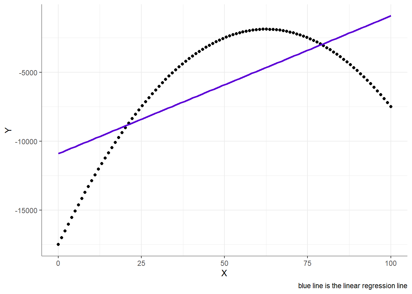
For example, when the relationship between a predictor ($X$) and an outcome ($Y$) is not linear:

This relationship is non linear, as in, the model of $Y=b_0+b_{1}X$ is incorrect. However, this does not mean that it is impossible to specify a linear model that will correctly estimate this non-linear relationship - we could, for instance, estimate the model $Y=b_0+b_{1}X+b_2{X}^2$. Though non-linear relationships can be modeled with linear regression, they still do require a linear outcome variable! A variable may be considered linear when a change of a certain size has the same meaning across the whole range of possible values of that variable. For example, a change from 3 to 6 should have the same meaning as a change from 21 to 24.¹ This is crucial as that is exactly what we are trying to model - differences (variance) in in the outcome. When an outcome is non-linear (see example below) the interpretation of linear models is at best an approximation, and at worst simply nonsensical.

The assumption of model-correctness is also violated by the addition or omission of variables in the model. For example, multicollinearity makes estimation of model parameters unstable, making the fitted model a bad estimate for the relationship between the predictors and the outcome variable. Likewise, by not include a mediator, moderator of covariate in your model, the model will misrepresent (either over- or under-estimate) the strength of relationship between $X$ and $Y$.

Note that this assumption is not violated if your variables are restricted / truncated / censored - having such variables does hinder your model’s ability to properly predict values outside this range, but it may still be a good (or even the best and most true) model for the range at hand.

What if this Assumption is Violated?

This is probably the most crucial assumption of linear regression, as there is no way to overcome its violation other than specifying the correct model. This might include adding or omitting variables in the model, or it might include using some non-linear models, such as a poisson or logistic regression (or others).

The bottom like here is that even if you find that the linear model is significant (even if it is “very significant”), that cannot and never will be enough to overcome the fact that the specified model - is wrong.

Part 2. Assumptions needed for NHST

Assuming you correctly fit your model, you now come to the dreaded part of testing its (or its covariates) significance, using an $F$- or $t$ null hypothesis significance test (NHST). These test require that the following 3 assumptions hold true:

1. Normality of residuals.
   
2. Independence of residuals.
   
3. Homoscedasticity of residuals.

But why? These assumptions are all needed since in significance tests we translate the ratio between the estimated parameter and its standard error to the probability of obtaining this ratio under the null hypothesis. This is done by looking up the cumulative probability of an estimated $F$-ratio under the $F$ distribution. But the distribution of possible $F$-ratios only takes the shape of the $F$-distribution when the residuals are independent from one another and are normally distributed (the same applies for the $t$-distribution).

Useless Data Transformations

But do you know what does not need to be normally distributed? Literally anything else! You can see this quite clearly when looking at the equation for $b_x$’s standard error:

$${\hat{S}}_b=\sqrt{\frac{\sum (y_i-\hat{y}{)}^2}{(N-k-1)}\cdot \frac{1}{\sum (x_i-\overline{x}{)}^2\cdot (1-R_x^2)}}$$

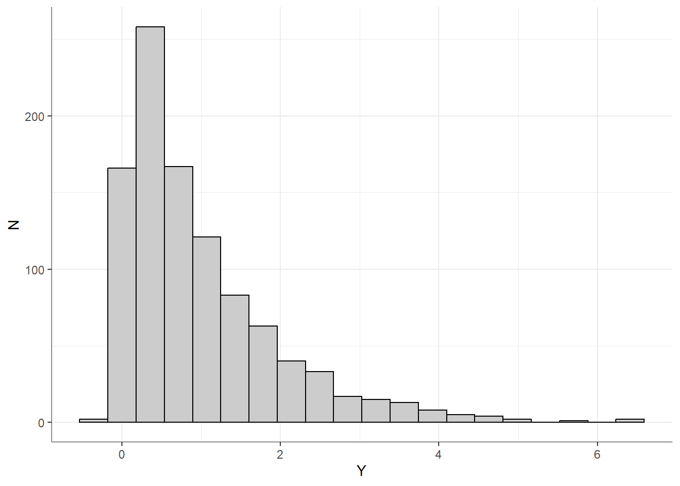
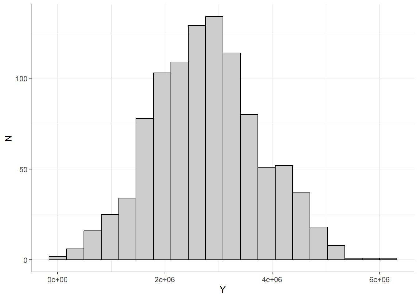
The left factor of the square-rooted term estimates the standard deviation of the residuals - the mean squared difference between the outcome and the predicted outcome. In other words, at no point in our modeling or NHST does the shape of the raw outcome or predictor(s) come into play (the right factor of the square-rooted term is simply a normalizing factor for the specific coefficient being tested). So for the love of Gauss, stop pointing out when variables are skewed, heavy tailed and the like. Only the shape of the residuals matters for this assumption to hold. For example, here we have a heavily skewed outcome variable:

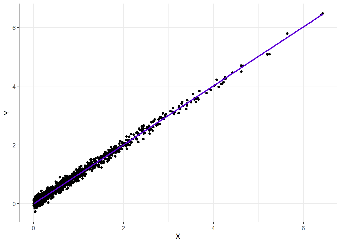
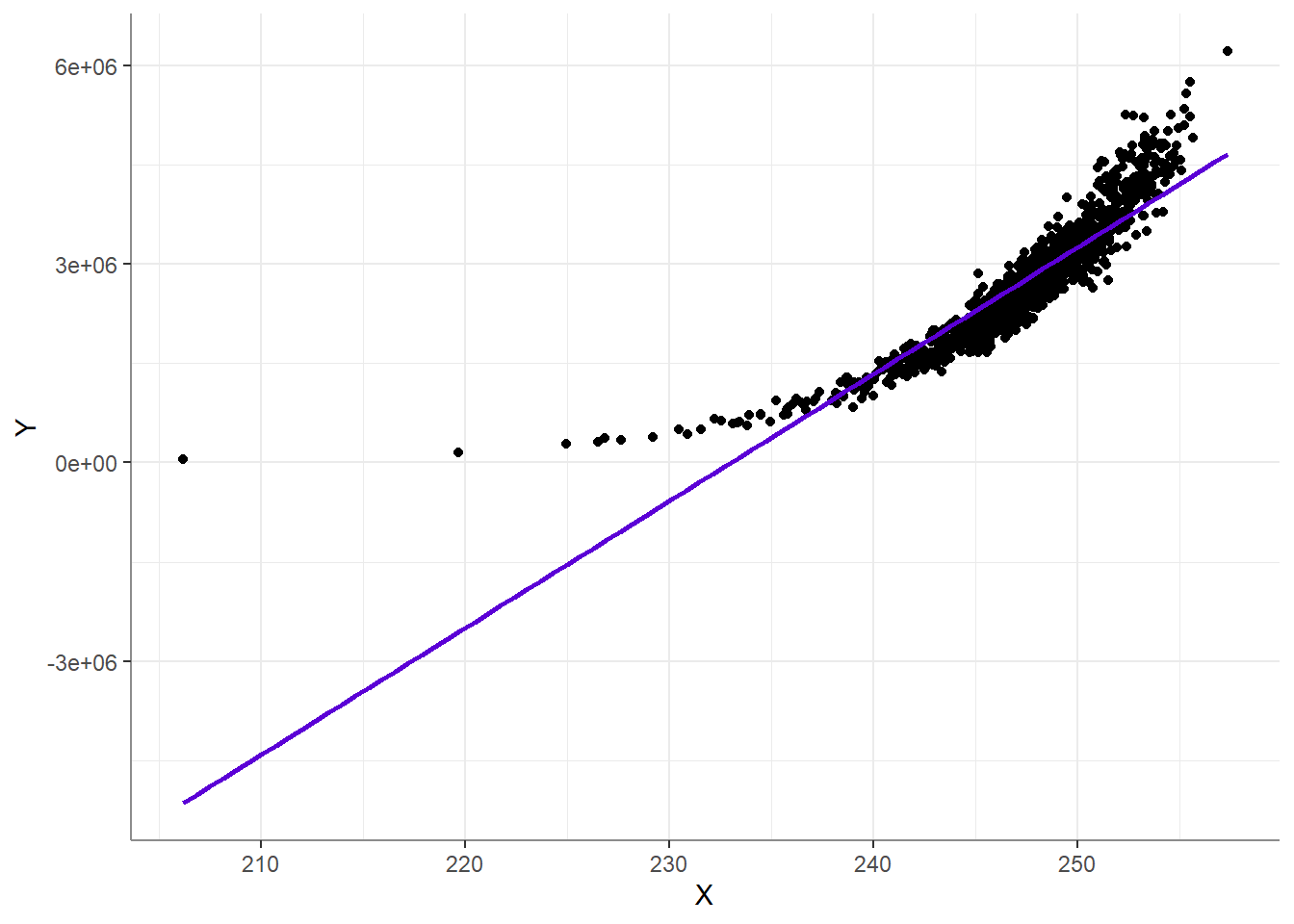
This seems alarming, maybe you’d want to combat this skewness with $log(x)$? But in fact, this is perfectly fine, as we can see when looking at the scatter plot:

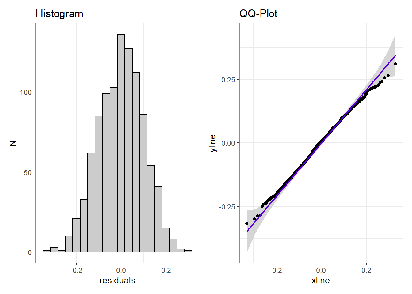
Or at the distribution of residuals:

On the other hand, if had you taken $log(x)$ to “combat” the skewness,

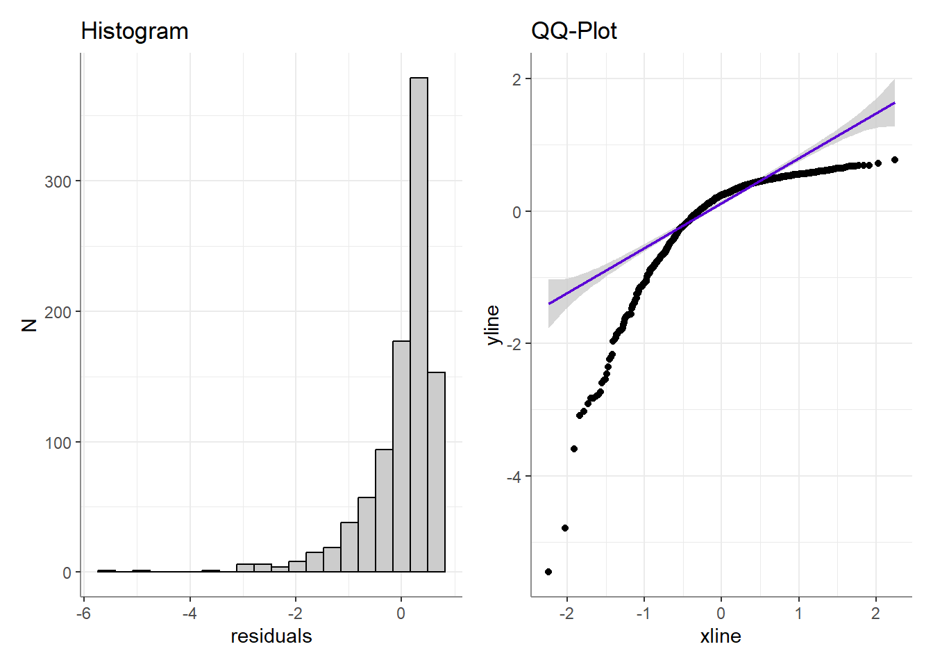
Oy vay… This is obviously an extreme example, but I make it to drive home the idea that robotically transforming skewed or heavy tailed variables is a bad habit. The only reason to ever transform a variable is if you think that by transforming the variable, you can properly represent its relationship with another variable in a linear model. For example, here we have a beautifully normally distributed outcome variable:

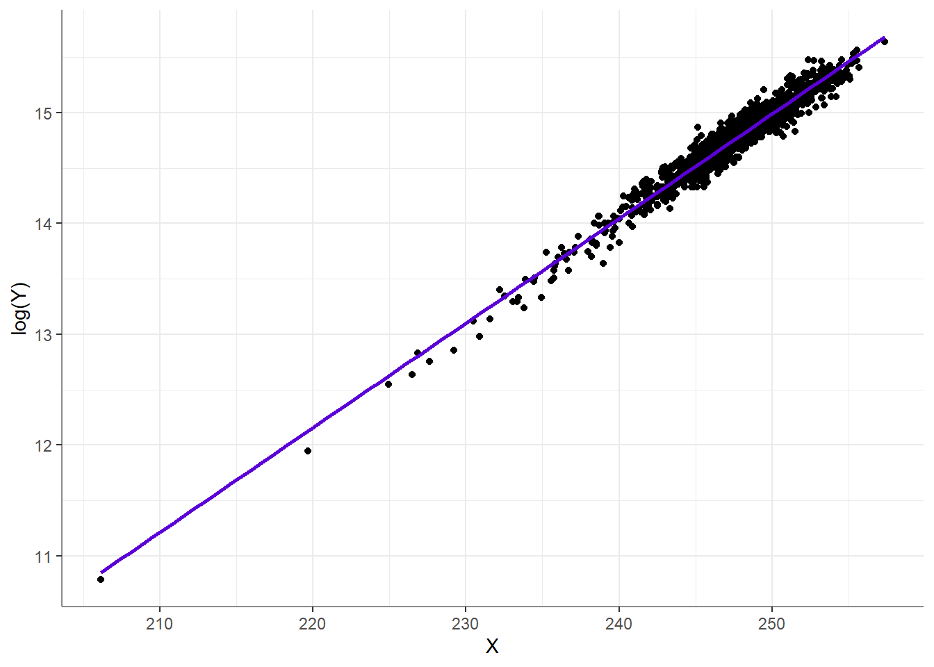
Yet when examining the relationship with a predictor, we find a non-linear relationship:

In this case, transforming $Y$ into $log(Y)$ is actually a good idea - and will give a linear model of an exponential relationship ($log(Y)=b_0+b_{1}X$)!

Heed my warning: transformations always change the pattern of the relationship between the outcome and the predictors. Use transformations only when needed, and avoid using them when someone points out that one of your predictors had high kurtosis they are not called for.

(Edit: Read and cite Adam M. Brickman’s excellent 2018 paper, and Andrew F. Hayes’s book (pp. 68-72) about this normalcy-fallacy).

Independence and Homoscedasticity

The independence of residuals is also needed for the proper translation of $F$- or $t$-ratios into probabilities, due to the underlying ${\chi }^2$ distribution. This is why un-modeled auto correlations are bad if not properly modeled in time-series data, as are dependent residuals due to repeated measure designs (which are accounted for and modeled in repeated measure / mixed-ANOVA / Linear mixed models).

Where does homoscedasticity (equality of variance) come into play? If we look back at the equation for $b_x$’s standard error, we can see that we are using all of the residuals to estimate a single ${\hat{S}}_e$. This is also apparent in the formal definition of the shape of distribution of residuals: $e\sim N(0,\sigma )$, we’re estimating the size of a single $\sigma$. Since we’re estimating a single error term, it would be inappropriate to do so based on heteroscedastic residuals (i.e., mixing residuals from differently scaled / shaped populations).

What if these Assumptions are Violated?

It is important to understand that if these assumptions are violated, they have absolutely no implications or effect on the correctness of your model. A linear model with heteroscedastic residuals is still a linear model (i.e., the conditional mean of $Y$ increases linearly as a function of $X$):

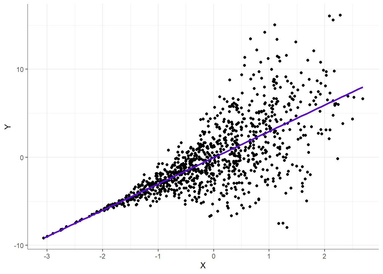
The only thing that is affected by the violations of these assumptions (any of them), is the ability to conduct NHST based on $F$ or $t$-ratios.² Put simply, the produced $p$-values, will simply not represent the probability of obtaining the results under the null hypothesis³. This can inflate false discovery rates, or extremely under-power your design (or the exact opposite, but let’s stay with the scare tactics for now).

So what can you do??

If you violate the assumption of independent residuals, improve your model - account for auto-correlations, or add a random intercept / slope to your model. Done!

If your residuals are not normally distributed or are heteroscedastic, you can use bootstrapping of permutation testing to conduct your NHST, and completely circumvent the need for these assumptions to hold!⁴

What About ANOVAs?

It should be noted that ANOVA $F$ tests and simple $t$ tests are special cases of regression (or of linear mixed models for repeated measure designs) where all the predictors are categorical, and thus everything said in this post can (and should) be applied to these analyses as well. In fact the normalcy-fallacy seems absurd when thinking of a simple $t$ test - how can a categorical predictor even be normally distributed?

Final Words

Teaching bad assumptions is bad. It is safe to assume that at least some published regression analyses violate some of the wrongfully taught incorrect assumptions. This means that while conducting these analyses at least some researchers, who held these false assumptions to be true, thought that they were doing something wrong or “statistically illegal” while they were actually being law abiding researchers. Who needs that kind of pressure?

Hopefully, after reading this, you are now equipped with the knowledge to conduct better analyses in the future, but most importantly, next time someone says that an assumption of regression is multivariate normality, you can snarkily reply “Um, actually, only the residuals need to be normally distributed…”.

---

Thanks to Tal Yatziv and Naama Yavor for reviewing this blog post before publication.

Footnotes

1. If this worried you, it should

2. If you’re fitting non-linear models - say, one of the family of GLM (such as logistic regression) - these assumption do not apply, because the test statistic ($z$ or ${\chi }^2$) do not require them. These models have different assumptions (can you say “overdispersion”?), but I’ll let someone else review those…

3. Though it is true that violating these assumptions has only a nominal effect on type-I errors, the effect on type-II errors can be substantive, and cause significant over estimations of study power. In either case, even though inference is robust to these violations, exact $p$-values cannot be reliably interpreted under such conditions (a practice that should be avoided anyway).

4. There are methods of correcting for heteroscedasticity, but they have their own sets of assumptions that can be violated. Recursive much?