Over a year ago, while listing to a very not-at-all-statistical podcast, I discovered that Bayesian modeling is widely used in archaeology since the mid 90s to calibrate carbon dating.1
Carbon dating is a scientific method used to determine the age of ancient artifacts and archaeological remains. It relies on the natural decay of a radioactive isotope called carbon-14, which is present in all living organisms. By measuring the amount of carbon-14 present in a sample, scientists can estimate its age with remarkable precision, over spans of thousands of years.
How do archaeologists calibrate carbon dating with Bayesian models? One way is by applying order constraints to their models.
In this post I will present what order constraints are, and how we may assess and apply them in Bayesian models using the {brms} package (Bürkner, 2017). I assume the reader is already somewhat familiar with the {brms} package, Bayesian modeling and core concepts in MCMC sampling.
I will be using the following packages and versions:
You will need the most recent development version of {posterior} for some of the code presented in this post. You can install it from GitHub by running the following:
The C14 column is the estimated carbon dating age (years before present, relative to today), and the error column provides the (estimated) measurement error in the C-14 assessment.
Our goal: to estimate the year from which each layer originates.
The Model
We will begin with an unassuming Gaussian model.
\[
\text{Carbon-14 Age}_i \sim N(\mu_i, \sigma^2 + \gamma^2_{ij}) \\
\] That is, each sample (with it’s own given measurement error \(\gamma^2_{ij}\)) comes from a layer with its own mean \(\mu_i\).
If this model doesn’t make sense to you, that’s because it’s only a partial model. Under the full model, each \(\mu\) is uniformly distributed:
\[
\mu_i \sim U(\alpha_i,\beta_i)
\]
With \(\alpha\) and \(\beta\) being the parameters of interest: marking the beginning and end of each layer.
We’ll set the following super-wide-and-very-weak priors:
\[
\mu_i \sim N(-5975, 1000)
\]
\[
\sigma \sim Exponential(0.01)
\]
In {brms}, this looks like this:
priors <-set_prior("normal(-5975, 1000)", class ="b") +set_prior("exponential(0.01)", class ="sigma")validate_prior(priors,bf(C14 |se(error, sigma =TRUE) ~0+ Layer),data = table1)#> prior class coef group resp dpar nlpar lb ub source#> normal(-5975, 1000) b user#> normal(-5975, 1000) b LayerB (vectorized)#> normal(-5975, 1000) b LayerC (vectorized)#> normal(-5975, 1000) b LayerE (vectorized)#> normal(-5975, 1000) b LayerG (vectorized)#> normal(-5975, 1000) b LayerI (vectorized)#> exponential(0.01) sigma 0 user
We can extract the posterior distribution of the \(\mu\) parameter from each layer using the posterior_linpred() function, or {tidybayes}’s add_linpred_*() function.
grid <-data.frame(Layer =c("B", "C", "E", "G", "I"),error =0)grid_with_mu <-add_linpred_rvars(grid, mod1, value =".mu")grid_with_mu#> # A tibble: 5 × 3#> Layer error .mu#> <chr> <dbl> <rvar[1d]>#> 1 B 0 -5671 ± 53#> 2 C 0 -5809 ± 63#> 3 E 0 -5894 ± 57#> 4 G 0 -6111 ± 64#> 5 I 0 -6295 ± 70
The .mu column contains a vector of class rvar – it is a convenient and tidy way to store samples of random variables, such as MCMC posterior draws.
Compare this to the “long” format, where each sample get’s its own row:
add_linpred_draws(grid, mod1, value =".mu")#> # A tibble: 20,000 × 7#> # Groups: Layer, error, .row [5]#> Layer error .row .chain .iteration .draw .mu#> <chr> <dbl> <int> <int> <int> <int> <dbl>#> 1 B 0 1 NA NA 1 -5737.#> 2 B 0 1 NA NA 2 -5552.#> 3 B 0 1 NA NA 3 -5578.#> 4 B 0 1 NA NA 4 -5576.#> 5 B 0 1 NA NA 5 -5710.#> 6 B 0 1 NA NA 6 -5635.#> 7 B 0 1 NA NA 7 -5675.#> 8 B 0 1 NA NA 8 -5646.#> 9 B 0 1 NA NA 9 -5647.#> 10 B 0 1 NA NA 10 -5662.#> # ℹ 19,990 more rows
CIs <-hdi(grid_with_mu$.mu)CIs$Parameter <- grid$Layer # Add the layer names backCIs#> Highest Density Interval#> #> Parameter | 95% HDI#> --------------------------------#> B | [-5771.10, -5563.86]#> C | [-5945.06, -5687.60]#> E | [-6008.23, -5780.24]#> G | [-6235.39, -5978.06]#> I | [-6427.16, -6152.16]
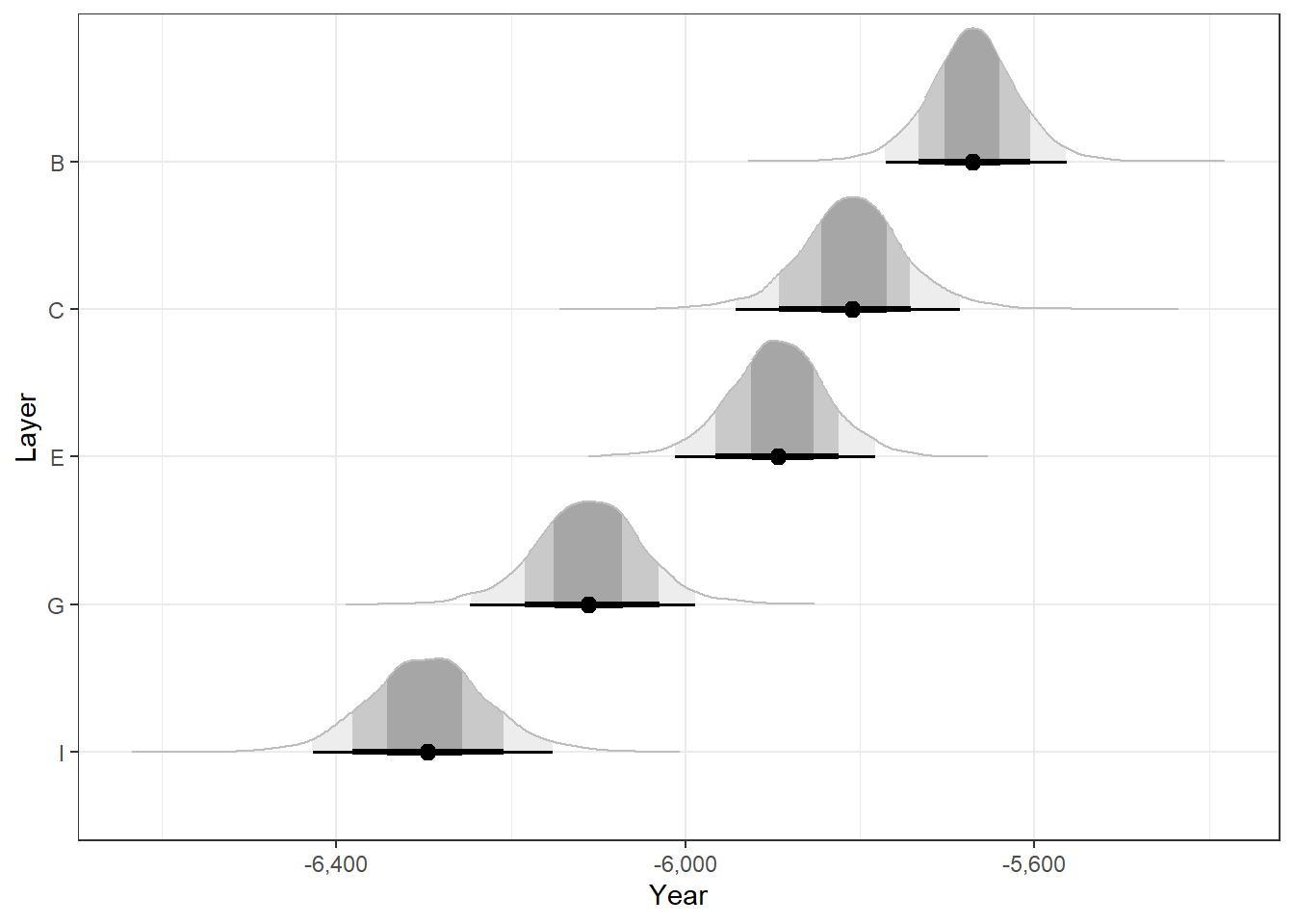
This model treats Layer as a categorical predictor: estimating the \(\mu\) parameter for each layer independently of the other layers. Of course we are happy to see that our basic knowledge of archaeology and time – specifically that layers are stratified: lower layers are older than the layers above them – is represented in the posterior.
But is it truly?
We can compute the posterior probability that the layers are in fact ordered. Once again, using rvars makes this relatively easy:
is_stratified is a logical rvar – TRUE for MCMC draws that conform to the ordering constraint, and FALSE for MCMC draws that do not.
The mean of these is the posterior probability of the constraint. Since this is a logical rvar, we can be fancy and use the Pr() function:
Pr(is_stratified)#> [1] 0.78725
That is, our posterior model strongly suggests that the layers are ordered, with a 0.79 posterior probability!
But we know a-priori that the layers are ordered! That is, the prior probability is 1, and therefore the posterior probability should also be 1! Can we incorporate this a-priori knowledge into our model / estimates?
What are Order Constraints?
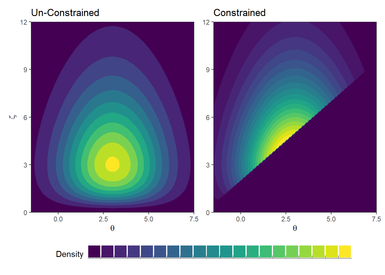
In Bayesian modeling, order constraints refer to restrictions imposed on the relationships between a model’s parameters. These constraints specify the order in which the parameters should appear or the direction of their relationships. For example, if we have the parameters \(\theta\), \(\gamma\) and \(\zeta\), the following are valid definitions of order constraints:
\((\theta > 3) \land (\gamma \geq \zeta)\) (\(\theta\) is greater than 3, AND \(\gamma\) is greater or equal to \(\zeta\))
\((\theta > \gamma) \lor \lnot (\theta > \zeta)\) (\(\theta\) is greater \(\gamma\) 3, OR \(\theta\) is NOT greater than \(\zeta\))
\((\theta - \zeta < 2) \land (\theta - \zeta > 0)\) (The difference between \(\theta\) and \(\zeta\) is less than 2 AND greater than 0.)
Etc…
These constraints are applied on top of any prior specification. This means that if we have the the following prior or posterior distribution defined by the following marginal distributions:
\[
\theta \sim Normal(3, 2)
\]
\[
\zeta \sim \chi^2(5)
\]
AND the constraint that \(\theta > \zeta - 2\), then the constrained distribution looks like this (on the right):
Plot Code
dens_grid <-expand_grid(tibble(x =seq(-1.5, 7.5, len =200),dx =dnorm(x, 3, 2, log =TRUE)),tibble(y =seq(0, 12, len =200),dy =dchisq(y, 5, log =TRUE)) ) |>mutate(d =exp(dx + dy),d = d /sum(d),d_c =replace(d, x > y -2, 0),d_c = d_c /sum(d_c) )p1 <-ggplot(dens_grid, aes(x, y, z = d)) +geom_contour_filled(breaks =seq(0, max(dens_grid$d_c), len =21)) +scale_x_continuous(expression(theta), expand =c(0, 0)) +scale_y_continuous(expression(zeta), expand =c(0, 0)) +guides(fill ="none") +labs(title ="Un-Constrained")p2 <- p1 +aes(z = d_c) +guides(fill =guide_bins(title ="Density", label =FALSE)) +theme(axis.title.y =element_blank()) +labs(title ="Constrained")patchwork::wrap_plots(p1, p2, guides ="collect") &theme(legend.position ="bottom")
Note that after applying the constraint, \(\theta\) and \(\zeta\)’s marginal distributions are different than those defined originally.
The application of order constraints in Bayesian modeling helps to incorporate prior knowledge and structural assumptions into the model. As we will see, by constraining the parameters, we can reduce the uncertainty in the model estimates and improve the interpretability of the results.
Back to our example - how can we apply the order constraints to our Layer data?
Constraining Post-Sampling
One solution for integrating a-priori model constraints into our posterior is to constrain our posterior model post-sampling simply by discarding any posterior draw that does not conform to our constraint.
Let’s denote the parameter space that is within our specified constrain as \(S_Y^k\)(borrowing the notation from the seminal work of Gelfand, Smith, & Lee, 1992). Had we constrained our model a-priori to \(S_Y^k\), what would be the effect on parameter values \(\theta\) that are outside the constrained \(S_Y^k\) space (\(\theta \notin S_Y^k\))? Their prior probability is 0. Therefore their posterior probability would also be 0.
What would be the effect of constraining our model a-priori on the probability of values within \(S_Y^k\) (\(\theta \in S_Y^k\))? Their prior probability distribution would have to be proportionally adjusted by \(1/p(S_Y^k)\) (the ratio of the unconstrained space to the constrained space). Since this value is a constant, the posterior probability is simply scaled by this amount.
For any MCMC sampler that only needs a function that is proportional to the posterior density function:
In other words, proportionally, applying the constraint is equivalent to simply not sampling outside of \(S_Y^k\) – or discarding any such samples.
We can keep only the samples within the constrained space by subsetting our posterior rvar with the is_stratifiedrvar! (This requires the {posterior} package, version 1.4.1.9000 at least.)
# subset with logical rvargrid_with_mu$.mu_constrained <- grid_with_mu$.mu[is_stratified]
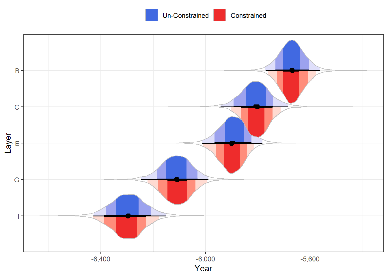
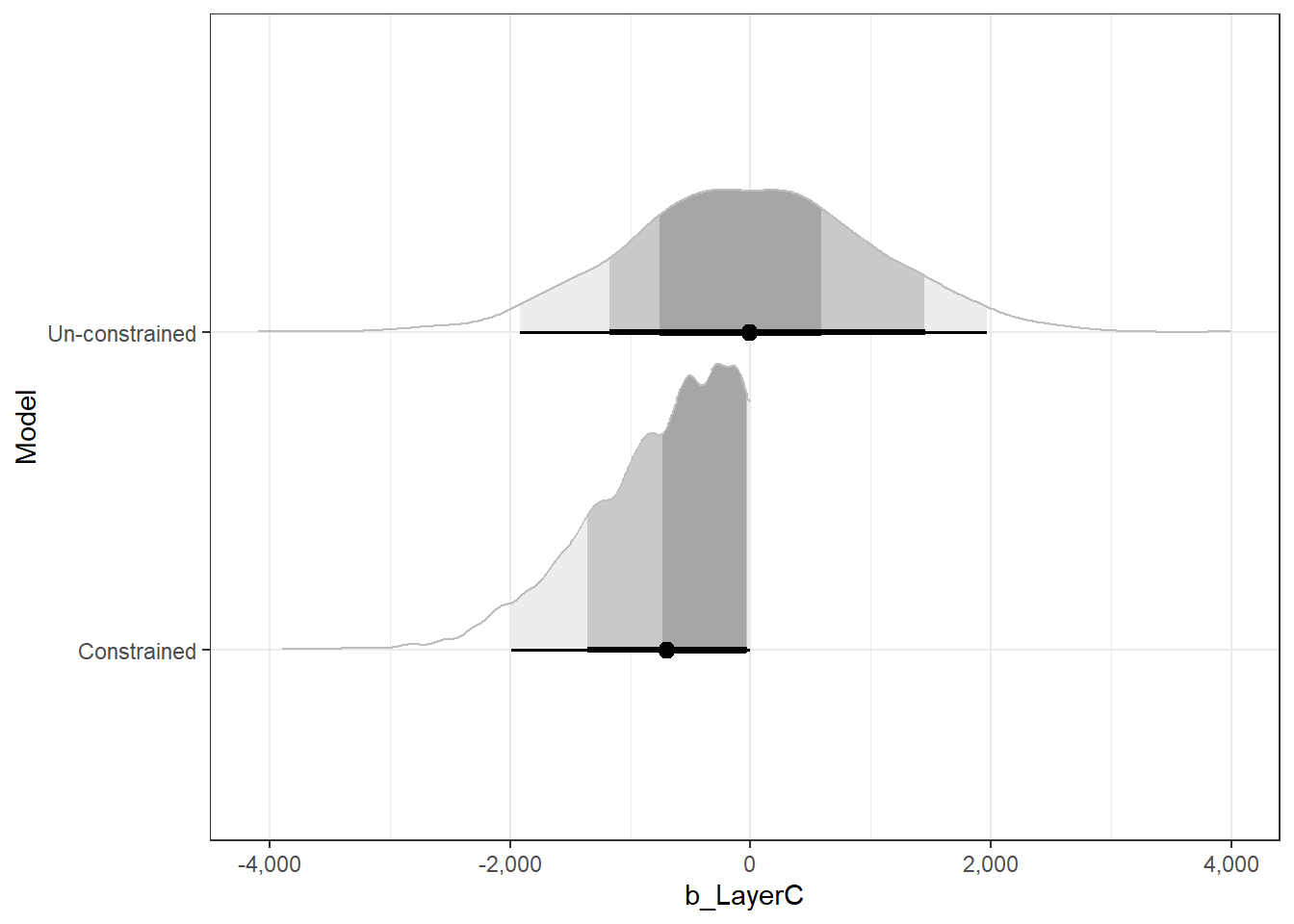
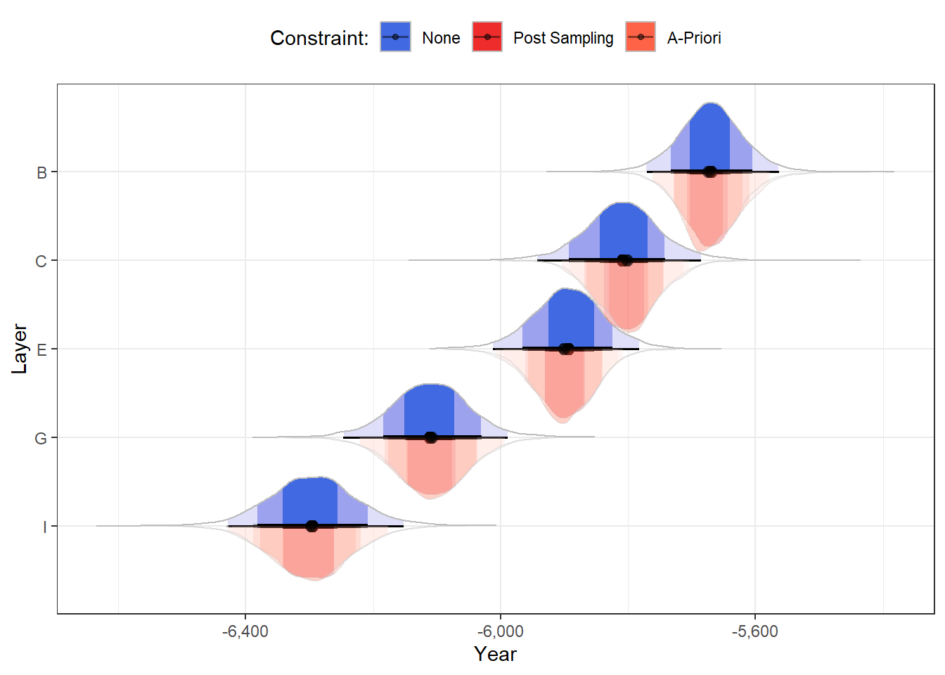
If we now plot our posteriors, we can see that the constrained posteriors are ever-so-slightly more narrow than the unconstrained ones, as if the edges of the samples are afraid to touch the adjacent layers’ posteriors:
Looking at the 95% HDI, we can see that we were able to shave a couple of decades off the CI boundaries (note especially how Layers C and E have shifted slightly away from each other).
CIs#> Highest Density Interval#> #> Parameter | 95% HDI#> --------------------------------#> B | [-5771.10, -5563.86]#> C | [-5945.06, -5687.60]#> E | [-6008.23, -5780.24]#> G | [-6235.39, -5978.06]#> I | [-6427.16, -6152.16]CIs_constrained <-hdi(grid_with_mu$.mu_constrained)CIs_constrained$Parameter <- grid$LayerCIs_constrained#> Highest Density Interval#> #> Parameter | 95% HDI#> --------------------------------#> B | [-5760.49, -5576.41]#> C | [-5902.04, -5711.58]#> E | [-6002.56, -5809.96]#> G | [-6222.13, -5994.23]#> I | [-6421.89, -6169.61]
This might not seem like much, especially considering the time scale we’re on. But imagine how crucial a decade in archaeological research can be! For example, one of the layers might contain a slab with the writing “… glory to king Jeroboam”, which unfortunately for you (my dear archaeologist) was a popular regal name in ancient Israel – there were two kings by the name of “Jeroboam” who lived within 130 years from each other; Narrowing a layer’s estimated C-14 year span can be crucial to dating the layer and its artifacts.
These post-sampling constraints can be applied to all brms() outputs (the various posterior_*(<brmsfit>) or {tidybayes}’s add_*() functions) by providing a vector of draw indices that conform to the constraint via the draw_ids argument.
i <-which(draws_of(is_stratified))
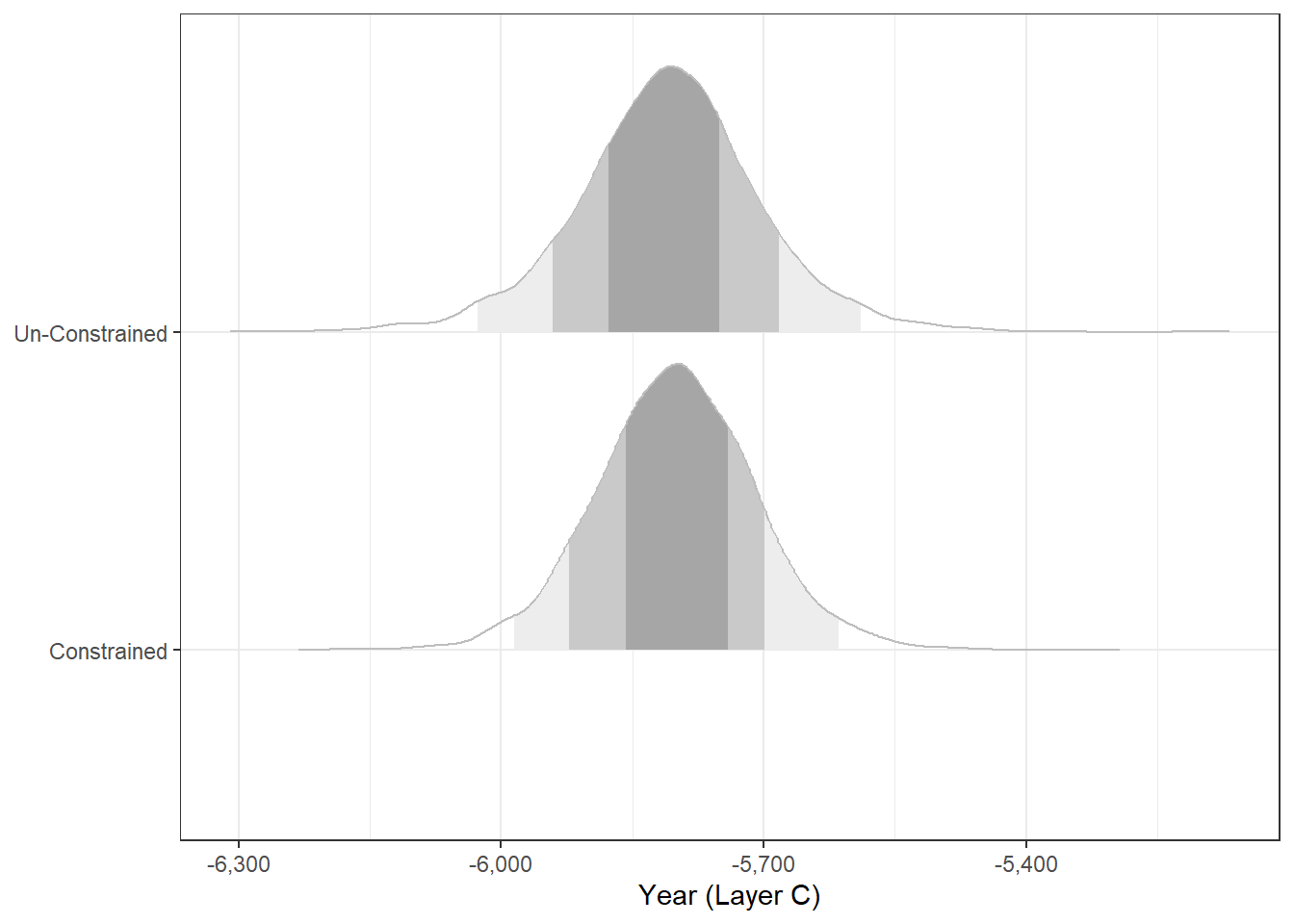
For example, we can obtain the PPD (posterior predictive distribution) for Layer C:
layerC <-data.frame(Layer ="C", error =0)layerC$PPD <-posterior_predict(mod1, newdata = layerC) |>rvar()layerC$PPD_constrained <-posterior_predict(mod1, newdata = layerC, draw_ids = i) |>rvar()# # Or with {tidybayes}:# layerC <- add_predicted_rvars(layerC, mod1, value = "PPD")# layerC <- add_predicted_rvars(layerC, mod1, value = "PPD_constrained", draw_ids = i)
The constrained model is slightly preferred \(\Delta LOOIC/SE_{\Delta} = 2.8\)!2 We can also test such constraints post-sampling with Bayes factors using {bayestestR}’s bayesfactor_restricted() (see the accompanying vignette).
These constraints can also be applied to estimates generated with {emmeans} or {marginaleffects}, again via the draw_ids argument (which can themselves be passed to the various {bayestestR} functions).
The constraints we’re using in this blog post involve all of the parameters which we are interested in estimating. But this need not be the case. For example, the constraint can be defined based one only a few parameters, and still apply it to all the parameters.
# Define constraint on mu_B, mu_C, mu_Gnew_constraint <-with(grid_with_mu, { .mu[Layer =="B"] > .mu[Layer =="C"] & .mu[Layer =="C"] - .mu[Layer =="G"] >150})Pr(new_constraint)#> [1] 0.90725# Apply constraint when estimating all parametersCIs_constrained2 <-hdi(grid_with_mu$.mu[new_constraint])CIs_constrained2$Parameter <- grid_with_mu$LayerCIs_constrained2#> Highest Density Interval#> #> Parameter | 95% HDI#> --------------------------------#> B | [-5765.22, -5573.01]#> C | [-5909.03, -5701.18]#> E | [-6001.42, -5780.24]#> G | [-6232.84, -5999.40]#> I | [-6429.44, -6164.50]
Constraining the Model A-Priori
Constraining post-sampling is wasteful: not only are we now estimating based on less samples, but our poor MCMC sampler worked so hard getting those 800~ samples we discarded. It sure would be great if we could constrain our model from the start.
priors <-set_prior("normal(-5975, 1000)", coef ="Intercept") +set_prior("normal(0, 1000)", class ="b") +set_prior("exponential(0.01)", class ="sigma")validate_prior(priors, bf(C14 |se(error, sigma =TRUE) ~0+ Intercept + Layer),data = table1)#> prior class coef group resp dpar nlpar lb ub source#> normal(0, 1000) b user#> normal(-5975, 1000) b Intercept user#> normal(0, 1000) b LayerC (vectorized)#> normal(0, 1000) b LayerE (vectorized)#> normal(0, 1000) b LayerG (vectorized)#> normal(0, 1000) b LayerI (vectorized)#> exponential(0.01) sigma 0 user
However, we would also like to add the following constraints:
Each of the Layer coefficients can only be negative.
and each coefficient is more negative than the coefficient of the layer above it.
Unfortunately, brms does not readily support such constraints. For example, if we try to constrain the LayerC coefficient to be negative by specifying the upper bound (ub) to be 0 we get the following error:
set_prior("normal(0, 1000)", class ="b", coef ="LayerC", ub =0)#> Error: Argument 'coef' may not be specified when using boundaries.
Alas, we need to write some Stan…. But only a little!
In Stan, we can define reject statements, which reject candidate values from being sampled. This is typically done conditionally. For example, we can test if b[1] (corresponding to b_LayerC) is positive, and reject the sample if it is.
if (!(b[2] < 0)) {reject("Hey! This value of b_LayerC is a-priori impossible!");}
Simple enough!
Luckily for us, brms is actually 100% powered by Stan – it converts our R-flavored model specifications, and translates them automagically into Stan. We can see the raw Stan code using the make_stancode() function:
make_stancode(bf(C14 |se(error, sigma =TRUE) ~0+ Intercept + Layer),data = table1, prior = priors)#> // generated with brms 2.19.0#> functions {#> #> }#> data {#> int<lower=1> N; // total number of observations#> vector[N] Y; // response variable#> vector<lower=0>[N] se; // known sampling error#> int<lower=1> K; // number of population-level effects#> matrix[N, K] X; // population-level design matrix#> int prior_only; // should the likelihood be ignored?#> }#> transformed data {#> vector<lower=0>[N] se2 = square(se);#> }#> parameters {#> vector[K] b; // population-level effects#> real<lower=0> sigma; // dispersion parameter#> }#> transformed parameters {#> real lprior = 0; // prior contributions to the log posterior#> lprior += normal_lpdf(b[1] | -5975, 1000);#> lprior += normal_lpdf(b[2] | 0, 1000);#> lprior += normal_lpdf(b[3] | 0, 1000);#> lprior += normal_lpdf(b[4] | 0, 1000);#> lprior += normal_lpdf(b[5] | 0, 1000);#> lprior += exponential_lpdf(sigma | 0.01);#> }#> model {#> // likelihood including constants#> if (!prior_only) {#> // initialize linear predictor term#> vector[N] mu = rep_vector(0.0, N);#> mu += X * b;#> target += normal_lpdf(Y | mu, sqrt(square(sigma) + se2));#> }#> // priors including constants#> target += lprior;#> }#> generated quantities {#> #> }#>
But brmsalso allows us to inject custom Stan code into the model before execution! And so, we can add such conditional reject statements, which are equivalent to setting the prior density of such values to 0 (=impossible).
svar <-stanvar(scode =' if (!(b[2] < 0)) { reject("Hey! This value of b_LayerC is a-priori impossible!"); } ', block ="tparameters")
We can see it injected into the Stan model, under the transformed parameters block:
make_stancode(bf(C14 |se(error, sigma =TRUE) ~0+ Intercept + Layer),data = table1, prior = priors, stanvars = svar)#> // generated with brms 2.19.0#> functions {#> #> }#> data {#> int<lower=1> N; // total number of observations#> vector[N] Y; // response variable#> vector<lower=0>[N] se; // known sampling error#> int<lower=1> K; // number of population-level effects#> matrix[N, K] X; // population-level design matrix#> int prior_only; // should the likelihood be ignored?#> }#> transformed data {#> vector<lower=0>[N] se2 = square(se);#> }#> parameters {#> vector[K] b; // population-level effects#> real<lower=0> sigma; // dispersion parameter#> }#> transformed parameters {#> real lprior = 0; // prior contributions to the log posterior#> #> if (!(b[2] < 0)) {#> reject("Hey! This value of b_LayerC is a-priori impossible!");#> }#> #> lprior += normal_lpdf(b[1] | -5975, 1000);#> lprior += normal_lpdf(b[2] | 0, 1000);#> lprior += normal_lpdf(b[3] | 0, 1000);#> lprior += normal_lpdf(b[4] | 0, 1000);#> lprior += normal_lpdf(b[5] | 0, 1000);#> lprior += exponential_lpdf(sigma | 0.01);#> }#> model {#> // likelihood including constants#> if (!prior_only) {#> // initialize linear predictor term#> vector[N] mu = rep_vector(0.0, N);#> mu += X * b;#> target += normal_lpdf(Y | mu, sqrt(square(sigma) + se2));#> }#> // priors including constants#> target += lprior;#> }#> generated quantities {#> #> }#>
Let’s see if it works by sampling from the prior distribution:
Let’s apply all of the constraints we want: we want the first “slope” to be negative, and then each consecutive slope to be more negative than the previous one. If one of these does not apply, we will reject the sample.
(We will use some inits here to make sure that our starting point for MCMC sampling is within our constrained space. Read more about those in Solomon Kurz’s excellent blog post.)
init <-list(# Give broad initial values that satisfy the order constraintsb =c(-5000, -100, -150, -200, -250))mod2_with_full_constrain <-brm(bf(C14 |se(error, sigma =TRUE) ~0+ Intercept + Layer),family =gaussian("identity"),prior = priors,stanvars = svar,data = table1,init =list(init, init, init, init),seed =1234)
Note that the Stan reference manual actually recommends against using reject statements in this way. Instead it advocates for writing out model constraints properly in parameter definitions and model parameterization. But hey, if we knew how to do that…
Additionally, the Stan user’s guide notes that applying such constraints on the prior-model does not allow us to assess the validity of the constraint (the posterior probability of the constraint in the unconstrained posterior model).
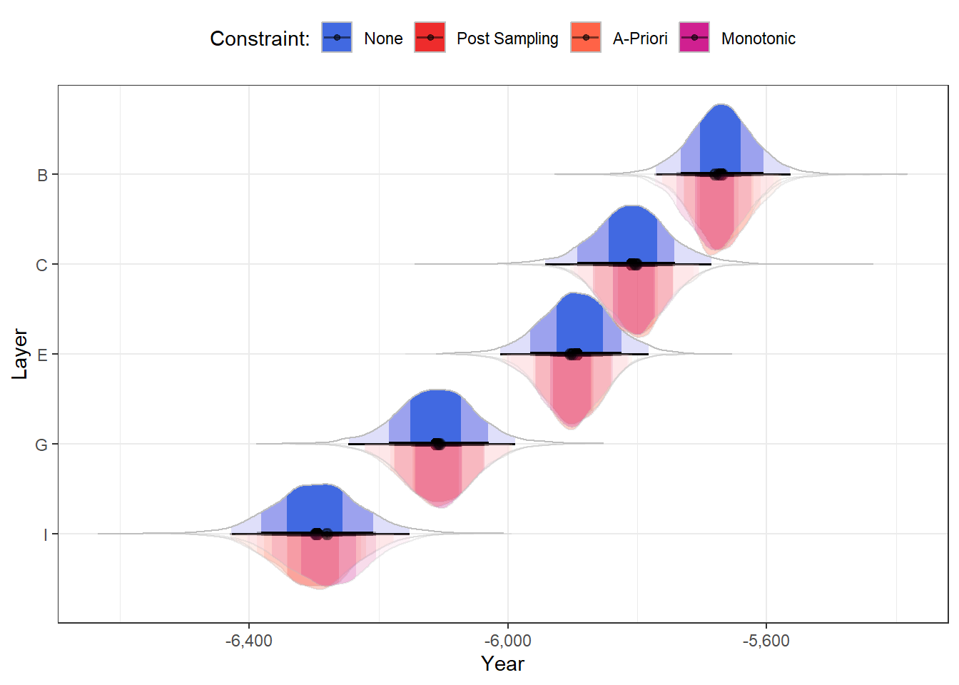
Monotonic Effects
What we’ve seen can be applied to any order constraints. However, the specific constraint we’re looking at here is a monotonic constraint, where the outcome exclusively increases or decreases from each consecutive level to the next (see Bürkner & Charpentier, 2020).
brms actually comes with a built-in function to do this: mo(). By using this in the model’s formula, brms parameterizes the model such that the monotonic effect is defined by two parameters:
A slope (b_moLayer) representing the direction and strength of the change.
A simplex (simo) defining the change increments from level to level.
get_prior(bf(C14 |se(error, sigma =TRUE) ~1+mo(Layer)),family =gaussian("identity"),data = table1)#> prior class coef group resp dpar nlpar lb ub#> (flat) b #> (flat) b moLayer #> student_t(3, -5883, 206.8) Intercept #> student_t(3, 0, 206.8) sigma 0 #> dirichlet(1) simo moLayer1 #> source#> default#> (vectorized)#> default#> default#> default
To apply this method we first need to recode the Layer predictor as an ordinal factor:
table1$Layer <-as.ordered(table1$Layer)
Using the same priors on the intercept and the variance, let’s fit the monotonic model.
priors <-set_prior("normal(-5975, 1000)", class ="Intercept") +set_prior("exponential(0.01)", class ="sigma")mod3_mo <-brm(bf(C14 |se(error, sigma =TRUE) ~1+mo(Layer)),family =gaussian("identity"),prior = priors,data = table1,seed =4321)
Although the mo() method does constrain the differences between levels to be monotonic, it does not constrain (a-priori) the direction of the differences. However, in this model, that is of no consequence – the posterior direction is completely negative:
Order constraints can be applied in a variety of models. For example, to examine if the direction of psychological effects is homogeneous (see Haaf & Rouder, 2017).
Such constraints can also be tested with Bayes factors – comparing the unconstrained model to the constrained model (and constrained model to any other model). Unlike other Bayes factors, these Order Bayes factors are not (as) sensitive to the width of (0-centered) priors, and often it is relatively straightforward to elicit order constraints from theoretical models (Heck, Wagenmakers, & Morey, 2015; Morey & Wagenmakers, 2014).
In this post we’ve seen how to define and apply such constraints a-priori and post-sampling. The consensus seems to be that post-sampling constraints are preferable – and here we’ve seen how easy it is to work with post-sampling constraints with post-sampling packages such as {posterior}, {ggdist}, {bayestestR}, {emmeans} and {marginaleffects}, as well as with post-sampling functions within {brms} itself.
Overall, order constraints are amazingly powerful tools to add to your Bayesian utility belt: they are easy – almost natural – to think about, and easy to implement (especially post-sampling). I hope you use them to unearth some new truths!
Hey, Thanks!
I’d like to thank Solomon Kurz (@SolomonKurz) for taking the time to review this post and for offering useful feedback.
Bürkner, P.-C. (2017). Brms: An r package for bayesian multilevel models using stan. Journal of Statistical Software, 80, 1–28. https://doi.org/10.18637/jss.v080.i01
Bürkner, P.-C., & Charpentier, E. (2020). Modelling monotonic effects of ordinal predictors in bayesian regression models. British Journal of Mathematical and Statistical Psychology, 73(3), 420–451. https://doi.org/10.1111/bmsp.12195
Gelfand, A. E., Smith, A. F., & Lee, T.-M. (1992). Bayesian analysis of constrained parameter and truncated data problems using gibbs sampling. Journal of the American Statistical Association, 87(418), 523–532. https://doi.org/10.1080/01621459.1992.10475235
Haaf, J. M., & Rouder, J. N. (2017). Developing constraint in bayesian mixed models. Psychological Methods, 22(4), 779–798. https://doi.org/10.1037/met0000156
Heck, D. W., Wagenmakers, E.-J., & Morey, R. D. (2015). Testing order constraints: Qualitative differences between bayes factors and normalized maximum likelihood. Statistics & Probability Letters, 105, 157–162. https://doi.org/10.1016/j.spl.2015.06.014
Morey, R. D., & Wagenmakers, E.-J. (2014). Simple relation between bayesian order-restricted and point-null hypothesis tests. Statistics & Probability Letters, 92, 121–124. https://doi.org/10.1016/j.spl.2014.05.010
Footnotes
It was a podcast about the ancient near east, in Hebrew, featuring the archaeologist Israel Finkelstein. Among the many interesting things Finkelstein said, he also blurted:
“… which we modeled with Bayesian methods, and found that…”
And that’s was it. No further details were provided.
This was enough to send me down a rabit hole – the end product of which is this blog post and the final lesson in my Bayesian Modeling course for undergrad statisticians.
The keen-eyed reader will also notice that the effective number of parameters (p_loo) is smaller – the constrained model, naturally, has fewer free parameters.)↩︎