Ordinal Regression as a Model for Signal Detection

R
statistics
code
ordinal regression
signal detection theory
Author

Mattan S. Ben-Shachar

Published

October 6, 2022

Preface

I was basically done with this blog post when I came across Matti Vuorre’s post on the same exact topic. Matti goes into all the details, and really the present post can be seen as a brief account of all the cool things the probit-approach-to-SDT can do. I’m only posting this here because I really like my plots 🤷


Previously, we’ve seen that for data from a binary decision signal detection task, we can use a probit binomial regression model (like a logistic regression, but with a probit link function) to estimate the two main parameters of signal detection theory (SDT): the sensitivity and the bias.

In this post I would like to show how this idea can be extended to multiple response SDT tasks by using an ordinal probit regression model.

The Data

Imagine the following task: after being presented with 20 images of dogs, you are presented with 300 new images of dogs, and you have to decide for each dog if it appeared in the training set (“Old”) or not (“New”).

In a binary decision task, you would simply indicate “New” or “Old”, but in this task you have multiple response options - from 1 to 6, with 1 = “Feels New” and 6 = “Feels Old”. We can call this scale a “feelings numbers” scale.

After going over all 30 photos, you have

STD_data
# A tibble: 12 × 3
   Truth Response        N
   <fct> <ord>       <dbl>
 1 New   Confidence1    35
 2 New   Confidence2    31
 3 New   Confidence3    26
 4 New   Confidence4    22
 5 New   Confidence5    19
 6 New   Confidence6    17
 7 Old   Confidence1    14
 8 Old   Confidence2    20
 9 Old   Confidence3    22
10 Old   Confidence4    27
11 Old   Confidence5    32
12 Old   Confidence6    35

Where N is the number of responses in each condition and response level.

Modeling with Classic SDT

We can use Siegfried Macho’s R code to extract the SDT parameters. In this case, they are:

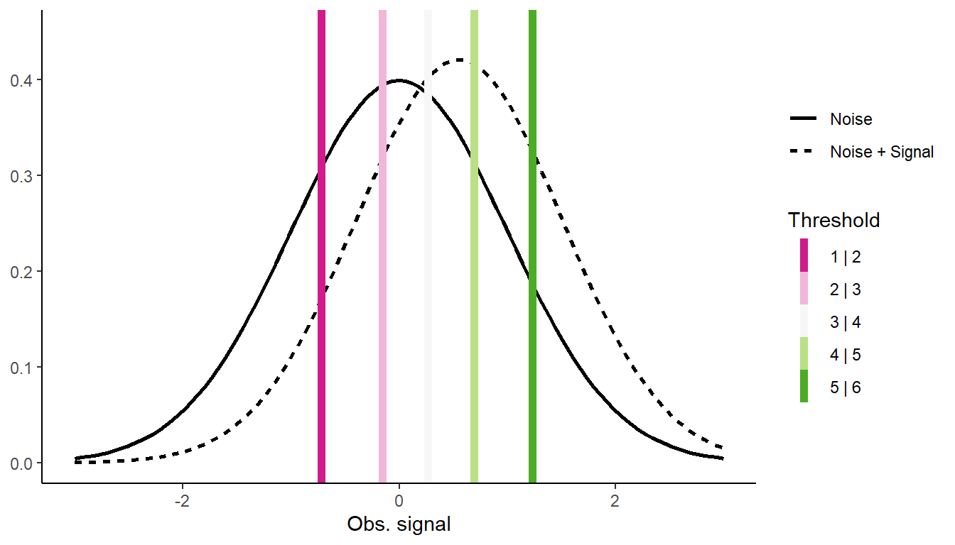
  1. Sensitivity - The distance between the two (latent) normal distributions. The further they are, the more “distinguishable” the Old and New images are from each other.
  2. 5 Threshold - One between each pair of consecutive possible responses. Perceived “stimulation” above each threshold leads to a decision in that category.

(These will probably make sense when we present them visually below.)

First, we’ll model this with classical SDT:

SDT_equal <- SDT.Estimate(
  data = STD_data[["N"]],
  test = TRUE,
  # We have 2 option: Old / New; We'll assume equal variance
  n = list(n.sdt = 2, restriction = "equalvar")
) 

SDT.Statistics(SDT_equal)[["Free.parameters"]]
         Value    SE CFI-95(Lower) CFI-95(Upper)
Mean[2]  0.564 0.040         0.486         0.642
t-1     -0.744 0.034        -0.810        -0.678
t-2     -0.165 0.031        -0.226        -0.104
t-3      0.267 0.031         0.206         0.329
t-4      0.707 0.033         0.643         0.772
t-5      1.260 0.036         1.189         1.331

Modeling as a Probit Cumulative Ordinal

library(dplyr)      # 1.1.4
library(tidyr)      # 1.3.0
library(ordinal)    # 2022.11.16
library(parameters) # 0.21.3
library(ggplot2)    # 3.4.4
library(patchwork)  # 1.1.3 

We can also model this data with a Probit Cumulative Ordinal model, predicting the Response from the Truth: - The slope of Truth indicates the effect of the true image identity had on the response pattern - this is sensitivity.
- In an ordinal model, we get k-1 “intercepts” (k being the number of unique responses). Each intercept represents the value above which a predicted value will be binned into the next class. There represent our shreshold.

m_equal <- clm(Response ~ Truth, 
  data = STD_data,
  weights = N,
  link = "probit"
)

parameters::model_parameters(m_equal) |> 
  insight::print_html()
Model Summary
Parameter Coefficient SE 95% CI z p
Intercept
Confidence1|Confidence2 -0.74 0.10 (-0.94, -0.54) -7.21 < .001
Confidence2|Confidence3 -0.16 0.10 (-0.35, 0.02) -1.72 0.085
Confidence3|Confidence4 0.27 0.10 (0.08, 0.46) 2.81 0.005
Confidence4|Confidence5 0.71 0.10 (0.51, 0.90) 7.08 < .001
Confidence5|Confidence6 1.26 0.11 (1.05, 1.48) 11.38 < .001
Location Parameters
Truth (Old) 0.57 0.12 (0.33, 0.81) 4.65 < .001

As we can see, the estimated values are identical!1

The advantage of the probit ordinal model is that it is easy(er) to build this model up:

  • Add predictors of sensitivity (interactions with Truth)
  • Add predictors of bias (main effects / intercept effects)
  • Add random effects (with ordinal::clmm())

(See Matti’s post for actual examples!)

mean2 <- coef(m_equal)[6]

Thresholds <- coef(m_equal)[1:5]

ggplot() + 
  # Noise
  stat_function(aes(linetype = "Noise"), fun = dnorm,
                linewidth = 1) + 
  # Noise + Signal
  stat_function(aes(linetype = "Noise + Signal"), fun = dnorm, 
                args = list(mean = mean2),
                linewidth = 1) + 
  # Thresholds
  geom_vline(aes(xintercept = Thresholds, color = names(Thresholds)),
             linewidth = 2) + 
  scale_color_brewer("Threshold", type = "div", palette = 2,
                     labels = paste0(1:5, " | ", 2:6)) + 
  labs(y = NULL, linetype = NULL, x = "Obs. signal") + 
  expand_limits(x = c(-3, 3), y = 0.45) + 
  theme_classic()

Unequal Variance

The standard model of SDT assumes that the Noise and the Noise + Signal distribution differ only in their mean; that is, N+S is a shifted N distribution. This is almost always not true, with \(\sigma_{\text{N+S}}>\sigma_{\text{N}}\).

To deal with this, we can also estimate the variance of the N+S distribution.

First, with the classic SDT model:

SDT_unequal <- SDT.Estimate(
  data = STD_data[["N"]],
  test = TRUE,
  # We have 2 option: Old / New; Not assuming equal variance
  n = list(n.sdt = 2, restriction = "no")
) 

SDT.Statistics(SDT_unequal)[["Free.parameters"]]
           Value    SE CFI-95(Lower) CFI-95(Upper)
Mean[2]    0.552 0.041         0.473         0.632
Stddev[2]  0.960 0.035         0.891         1.029
t-1       -0.728 0.036        -0.799        -0.658
t-2       -0.159 0.032        -0.221        -0.097
t-3        0.266 0.031         0.205         0.327
t-4        0.696 0.034         0.629         0.763
t-5        1.235 0.043         1.151         1.318

And with a probit ordinal regression, but allow the latent scale to vary:

m_unequal <- clm(Response ~ Truth, 
  scale = ~ Truth, # We indicate that the scale is a function of the underlying dist
  data = STD_data, 
  weights = N,
  link = "probit"
)

parameters::model_parameters(m_unequal) |> 
  insight::print_html()
Model Summary
Parameter Coefficient SE 95% CI z p
Intercept
Confidence1|Confidence2 -0.72 0.11 (-0.93, -0.50) -6.51 < .001
Confidence2|Confidence3 -0.16 0.10 (-0.34, 0.03) -1.61 0.107
Confidence3|Confidence4 0.27 0.10 (0.08, 0.45) 2.80 0.005
Confidence4|Confidence5 0.69 0.10 (0.49, 0.90) 6.66 < .001
Confidence5|Confidence6 1.23 0.13 (0.98, 1.49) 9.50 < .001
Location Parameters
Truth (Old) 0.55 0.12 (0.31, 0.80) 4.49 < .001
Scale Parameters
Truth (Old) -0.05 0.12 (0.31, 0.80) 4.49 < .001

The scale parameter needs to be back transformed to get the sd of the N+S distribution: \(e^{-0.05}=0.95\), and so one again the estimated values are identical!

mean2 <- coef(m_unequal)[6]
sd2 <- exp(coef(m_unequal)[7])

Thresholds <- coef(m_unequal)[1:5]

ggplot() + 
  # Noise
  stat_function(aes(linetype = "Noise"), fun = dnorm,
                linewidth = 1) + 
  # Noise + Signal
  stat_function(aes(linetype = "Noise + Signal"), fun = dnorm, 
                args = list(mean = mean2, sd = sd2),
                linewidth = 1) + 
  # Thresholds
  geom_vline(aes(xintercept = Thresholds, color = names(Thresholds)),
             linewidth = 2) + 
  scale_color_brewer("Threshold", type = "div", palette = 2,
                     labels = paste0(1:5, " | ", 2:6)) + 
  labs(y = NULL, linetype = NULL, x = "Obs. signal") + 
  expand_limits(x = c(-3, 3), y = 0.45) + 
  theme_classic()

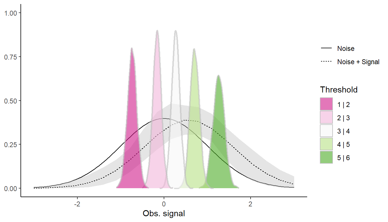
SDT with N and N+S distributions, and the 5 thresholds.

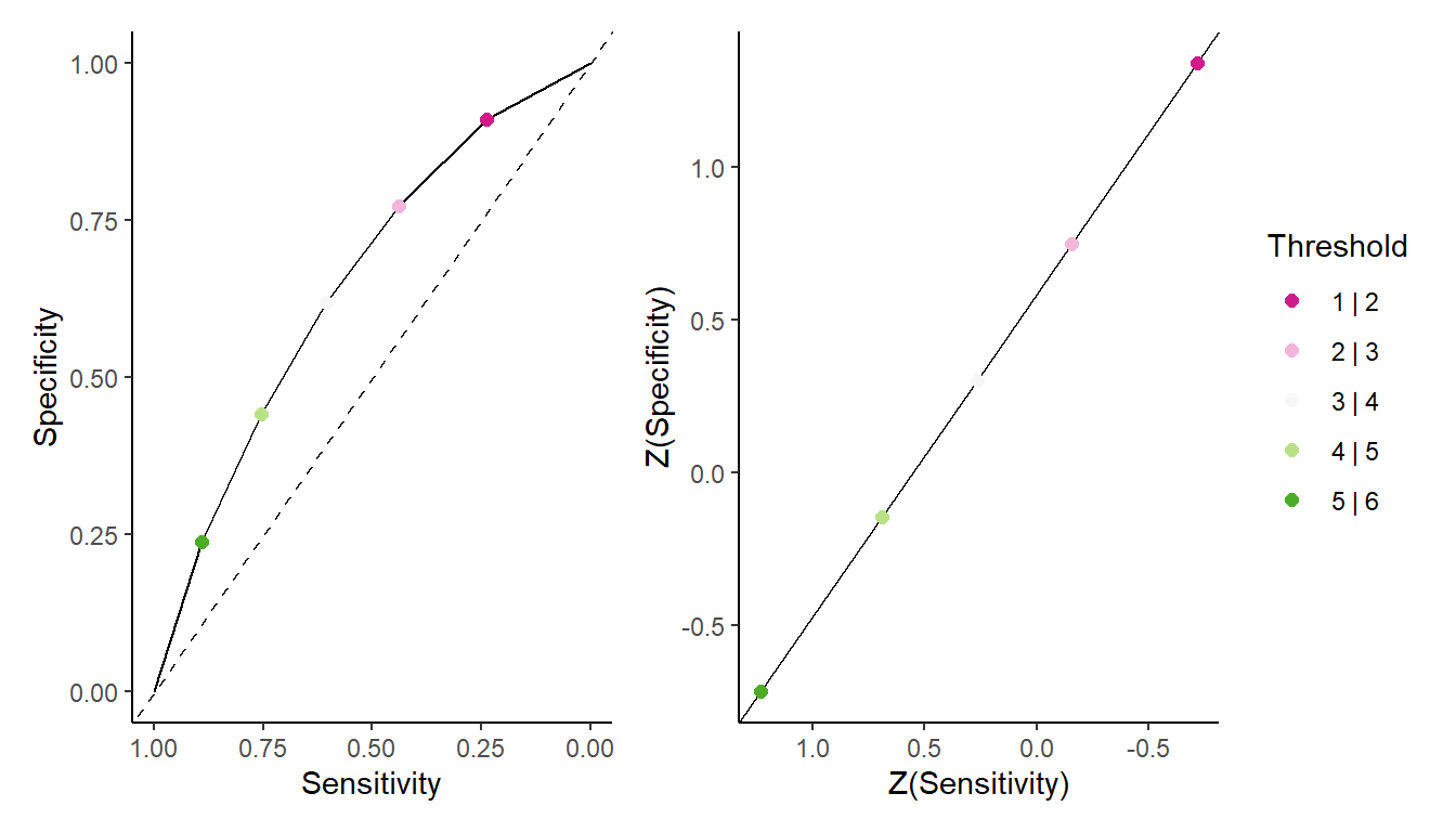
ROC Curve or ROC Curves?

An additional check we can preform is whether the various responses are indeed the product of single ROC curve. We do this by plotting the ROC curve on a inv-normal transformation (that is, converting probabilities into normal quantiles). Quantiles that fall on a straight line indicate they are part of the same curve.

pred_table <- data.frame(Truth = c("Old", "New")) |> 
  mutate(predict(m_unequal, newdata = pick(everything()), type = "prob")[[1]] |> as.data.frame()) |> 
  tidyr::pivot_longer(starts_with("Confidence"), names_to = "Response") |> 
  tidyr::pivot_wider(names_from = Truth)

ROC_table <- pred_table |> 
  mutate(
    Sensitivity = lag(cumsum(New), default = 0),
    Specificity = rev(cumsum(rev(Old))),
  ) |> 
  # Some clean up...
  rows_append(data.frame(Sensitivity = 1, Specificity = 0)) |> 
  mutate(
    Threshold = c(NA, paste0(1:5, "|", 2:6), NA)
  )

p_roc <- ggplot(ROC_table, aes(Sensitivity, Specificity)) + 
  geom_line() + 
  geom_abline(slope = 1, intercept = 1, linetype = "dashed") + 
  geom_point(aes(color = ordered(Threshold)), size = 2) + 
  expand_limits(x = c(0,1), y = c(0,1)) +
  scale_x_continuous(trans = "reverse") +
  scale_color_brewer("Threshold", type = "div", palette = 2,
                     labels = paste0(1:5, " | ", 2:6),
                     na.translate = FALSE) + 
  labs(color = NULL) + 
  theme_classic()

p_zroc <- ROC_table |> 
  ggplot(aes(qnorm(Sensitivity), qnorm(Specificity))) + 
  geom_line() + 
  geom_point(aes(color = ordered(Threshold)), size = 2) + 
  expand_limits(x = c(0,1), y = c(0,1)) +
  scale_x_continuous(trans = "reverse") +
  scale_color_brewer("Threshold", type = "div", palette = 2,
                     labels = paste0(1:5, " | ", 2:6),
                     na.translate = FALSE) + 
  labs(color = NULL, x = "Z(Sensitivity)", y = "Z(Specificity)") + 
  theme_classic()

p_roc + p_zroc + plot_layout(guides = "collect")
Warning: Removed 2 rows containing missing values (`geom_point()`).
Removed 2 rows containing missing values (`geom_point()`).

Because the point (on the Z-scale) fall on a straight line, we can confidently say they represent the same ROC curve.

Going Full Bayesian

Although the clmm() function allows for multilevel probit regression, it does not2 support varying scale parameter.

Alas, we must use brms.

library(brms)      # 2.20.4
library(ggdist)    # 3.3.1.9000
library(tidybayes) # 3.0.6 

In brms we will use the cumulative() family, which has a family-parameter called disc which gives the standard deviation of the latent distributions. I will set some weak priors on the mean and standard deviation of the N+S distribution, and I will also set the standard deviation of the N distribution to 1 (on a log scale, to 0) using the constant(0) prior.

b_formula <- bf(Response | weights(N) ~ Truth,
                disc ~ 0 + Intercept + Truth)
b_priors <- 
  set_prior("normal(0, 3)", coef = "TruthOld") + 
  set_prior("normal(0, 1.5)", coef = "TruthOld", dpar = "disc") + 
  set_prior("constant(0)", coef = "Intercept", dpar = "disc")


Bayes_mod <- brm(b_formula,
  prior = b_priors,
  family = cumulative(link = "probit", link_disc = "log"),
  data = STD_data,
  backend = "cmdstanr",
  refresh = 0
)
model_parameters(Bayes_mod, test = NULL) |> 
  insight::print_html()
Model Summary
Parameter Median 95% CI Rhat ESS
Intercept(1) -0.74 (-0.95, -0.52) 1.000 2799.00
Intercept(2) -0.16 (-0.36, 0.03) 1.000 4556.00
Intercept(3) 0.27 (0.08, 0.46) 1.000 5326.00
Intercept(4) 0.70 (0.50, 0.92) 1.000 4285.00
Intercept(5) 1.26 (1.01, 1.52) 1.000 2820.00
TruthOld 0.57 (0.32, 0.82) 1.000 3627.00
disc_Intercept 0.00 (0.00, 0.00)
disc_TruthOld 0.02 (-0.20, 0.24) 1.000 2068.00
criteria <- gather_rvars(Bayes_mod, b_Intercept[Response])

signal_dist <- spread_draws(Bayes_mod, b_TruthOld, b_disc_TruthOld) |>
  mutate(b_disc_TruthOld = exp(b_disc_TruthOld)) |>
  group_by(.draw) |>
  reframe(
    x = seq(-3, 3, length = 20),
    d = dnorm(x, mean = b_TruthOld, b_disc_TruthOld)
  ) |>
  ungroup() |>
  curve_interval(.along = x, .width = 0.9)

ggplot() +
  # Noise
  stat_function(aes(linetype = "Noise"), fun = dnorm) +
  # Noise + Signal
  geom_ribbon(aes(x = x, ymin = .lower, ymax = .upper),
              data = signal_dist,
              fill = "grey", alpha = 0.4) +
  geom_line(aes(x, d, linetype = "Noise + Signal"), data = signal_dist) +
  # Thresholds
  stat_slab(aes(xdist = .value, fill = ordered(Response)),
            color = "gray", alpha = 0.6, key_glyph = "polygon",
            data = criteria) +
  # Theme and scales
  scale_fill_brewer("Threshold", type = "div", palette = 2,
                     labels = paste0(1:5, " | ", 2:6),
                     na.translate = FALSE) + 
  labs(color = NULL, linetype = NULL, x = "Obs. signal", y = NULL) +
  theme_classic()

This gives roughly the same results as clm(), but would allow for multilevel modeling of both the location and scale of the latent variable.