`geom_smooth()` using formula = 'y ~ x'
`geom_smooth()` using formula = 'y ~ x'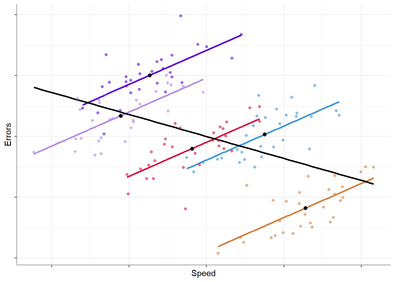
This is a comment on Solomon Kurz’s (@SolomonKurz) recent post1 where he discusses how group-level data does not always reflect individual-level processes. I highly recommend reading his series of posts on the topic!
In this post I will demonstrate:
Let’s work with the now-classic typing speed example. We take a group of 5 typists, and measure the speed of their typing (words per minute), and the rate of typing errors (errors per 100-words). Looking at the data we might get something like this:
`geom_smooth()` using formula = 'y ~ x'
`geom_smooth()` using formula = 'y ~ x'
As we can see, we have two sources of variation that can be used to explain or predict the rate of errors:
We can model these using liner mixed models, but first we need to split our predictor (speed) into two variables, each representing a different source of variance - each typist’s average typing speed, and the deviation of each measurement from the typist’s overall mean:2
library(dplyr)
data <- data %>%
  group_by(ID) %>%
  mutate(speed_M = mean(speed),
         speed_E = speed - speed_M) %>%
  ungroup()

head(data)
# A tibble: 6 × 5
ID speed errors speed_M speed_E
<int> <dbl> <dbl> <dbl> <dbl>
1 1 -0.773 -1.74 -0.188 -0.585
2 1 -0.144 -0.703 -0.188 0.0438
3 1 -0.686 -1.73 -0.188 -0.498
4 1 0.560 1.17 -0.188 0.748
5 1 0.214 0.316 -0.188 0.402
6 1 0.179 0.392 -0.188 0.367 Let’s fit a liner mixed model and see how we can detect both patterns correctly.
library(lmerTest)

fit <- lmer(errors ~ speed_M + speed_E + (1 + speed_E | ID),
            data = data)
Your model may suffer from singularity (see see `?lme4::isSingular` and
`?performance::check_singularity`).
Some of the standard errors and confidence intervals of the random
effects parameters are probably not meaningful!| Parameter | Coefficient | SE | CI | CI_low | CI_high | t | df_error | p | Effects | Group |
|---|---|---|---|---|---|---|---|---|---|---|
| (Intercept) | 0.000 | 0.620 | 0.95 | -1.225 | 1.225 | 0.000 | 143 | 1.000 | fixed | |
| speed_M | -1.600 | 0.693 | 0.95 | -2.969 | -0.231 | -2.309 | 143 | 0.022 | fixed | |
| speed_E | 1.400 | 0.119 | 0.95 | 1.165 | 1.635 | 11.762 | 143 | 0.000 | fixed | |
| SD (Intercept) | 1.379 | 0.568 | 0.95 | 0.615 | 3.093 | NA | NA | NA | random | ID |
| SD (speed_E) | 0.000 | 49027.294 | 0.95 | 0.000 | Inf | NA | NA | NA | random | ID |
| Cor (Intercept~speed_E) | 1.000 | 297941.433 | 0.95 | NaN | 1.000 | NA | NA | NA | random | ID |
| SD (Observations) | 0.717 | 0.043 | 0.95 | 0.637 | 0.806 | NA | NA | NA | random | Residual |
As we can see, the slope for speed_M is negative (-1.6), reflecting the group-level pattern where typists who are overall faster have fewer errors; whereas the slope for speed_E is positive (1.4), reflecting the individual-level pattern where faster typing leads to more errors.
Experiments!
Or to be more precise, when we control the values of the independent variable. Why is this so? Because we control the values of the independent variable, the independent variable cannot be split into different sources of variance: there is either variance between subjects (the variable is manipulated in a between-subjects design) or there is variance within subjects (the variable is manipulated in a within-subjects design), but never both. Thus, although there can be huge heterogeneity in the way subjects present an effect, the average individual-level effect will be the same as the group-level effect (depending on the design).3
and the short twitter discussion that followed.↩︎
Read more in: Hoffman, L. (2015). Time-varying predictors in models of within-person fluctuation. In Longitudinal analysis: Modeling within-person fluctuation and change (pp. 327-392). Routledge.↩︎
Ignoring any differences or artifacts that may arise from the differences in the design itself, such as order effects, etc.↩︎