Code
library(tidyverse)
library(patchwork)
library(gt)

# sysfonts::font_add_google(name = "fira code")
# showtext::showtext_auto()

knitr::opts_chunk$set(collapse = TRUE, comment = "#>", dev = "ragg_png")library(tidyverse)
library(patchwork)
library(gt)
# sysfonts::font_add_google(name = "fira code")
# showtext::showtext_auto()
knitr::opts_chunk$set(collapse = TRUE, comment = "#>", dev = "ragg_png")In celebration of the release of {ggplot2} 4.0.0 🥳, I wanted to explore the relationships between the geometric objects (“geoms”) and statistical transformations (“stats”) that are offered by the core {ggplot2} functions.
Within The Layered Grammar of Graphics framework, plots in {ggplot2} are built by adding layer()s. Each layer() consists of a geom (the actual thing being drawn), with different geoms having different aes()thetics that can (and should) be mapped to variables in the data.
However, all layer()s also have a stat - this can be thought of as a function applied to the data, transforming it in some way before it is passed to the geom and its aesthetics.
For example, geom_histogram() uses the "bin" stat by default:
geom_histogram()$stat
#> <ggproto object: Class StatBin, Stat, gg>
#>     aesthetics: function
#>     compute_group: function
#>     compute_layer: function
#>     compute_panel: function
#>     default_aes: ggplot2::mapping, uneval, gg, S7_object
#>     dropped_aes: weight
#>     extra_params: na.rm orientation
#>     finish_layer: function
#>     non_missing_aes:
#>     optional_aes:
#>     parameters: function
#>     required_aes: x|y
#>     retransform: TRUE
#>     setup_data: function
#>     setup_params: function
#>     super:  <ggproto object: Class Stat, gg>
This stat takes the raw data, counts the number of occurrences of each value of the x aesthetic within each x-bin.
p1 <- ggplot(mpg, aes(hwy)) +
  geom_histogram(bins = 10, color = "black")

p1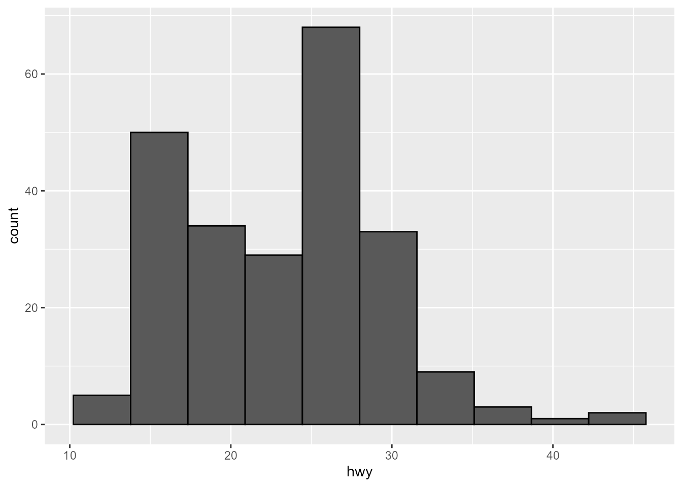
We can see the product of this transformation by using the layer_data() function, which extracts the data after it has been transformed by the stat:
# access the data from the first (and only) layer
layer_data(p1, i = 1) |>
  # see computed variables:
  select(x, count, density, ncount, ndensity, width)
#>           x count     density     ncount   ndensity width
#> 1  12.00000     5 0.006009615 0.07352941 0.07352941   0.9
#> 2  15.55556    50 0.060096154 0.73529412 0.73529412   0.9
#> 3  19.11111    34 0.040865385 0.50000000 0.50000000   0.9
#> 4  22.66667    29 0.034855769 0.42647059 0.42647059   0.9
#> 5  26.22222    68 0.081730769 1.00000000 1.00000000   0.9
#> 6  29.77778    33 0.039663462 0.48529412 0.48529412   0.9
#> 7  33.33333     9 0.010817308 0.13235294 0.13235294   0.9
#> 8  36.88889     3 0.003605769 0.04411765 0.04411765   0.9
#> 9  40.44444     1 0.001201923 0.01470588 0.01470588   0.9
#> 10 44.00000     2 0.002403846 0.02941176 0.02941176   0.9
We can see that this data has been transformed, and reflects the underlying data represented in the final plot in Figure 1: 10 columns, their x location, and their heights (count).1
Let’s take a deeper look at the geoms and stats in {ggplot2} and how they relate to each other.
# list all functions in ggplot2 that start with geom_ or stat_:
get_statgeom <- function(fname) {
  layer <- match.fun(fname)()
  data.frame(
    stat = class(layer$stat)[1],
    geom = class(layer$geom)[1]
  )
}

has_statgeom.args <- function(fname) {
  frmls <- formals(match.fun(fname))
  data.frame(
    has_stat_arg = "stat" %in% names(frmls),
    has_geom_arg = "geom" %in% names(frmls)
  )
}

ggdata <- data.frame(
  ggfunction = ls("package:ggplot2", pattern = "^(geom|stat)_")
) |>
  filter(
    !str_detect(ggfunction, "(bin2d|density2d|binhex|summary2d)"),
    !ggfunction %in% c("geom_errobarh")
  ) |>
  mutate(
    type = case_when(
      str_starts(ggfunction, "geom_") ~ "geom",
      str_starts(ggfunction, "stat_") ~ "stat",
      TRUE ~ NA_character_
    ),

    help_page = map(ggfunction, help) |>
      map(as.character) |>
      map_chr(str_extract, "(?<=help/).*"),

    map(ggfunction, possibly(get_statgeom, data.frame(NA))) |>
      bind_rows(),

    map(ggfunction, has_statgeom.args) |>
      bind_rows()
  ) |>
  select(-`NA.`) |>
filter(!(is.na(stat) & is.na(geom)), !help_page %in% c("ggsf"))ggdata_tidy <- ggdata |>
mutate(
stat = str_remove(stat, "Stat") |> str_to_lower(),
geom = str_remove(geom, "Geom") |> str_to_lower(),
stat = fct_reorder(factor(stat), stat, .fun = length),
geom = fct_reorder(factor(geom), stat, .fun = length)
)
ggplot(ggdata_tidy, aes(geom, stat)) +
geom_point() +
scale_x_discrete(limits = rev, guide = guide_axis(angle = -40)) +
theme(text = element_text(family = "fira code"))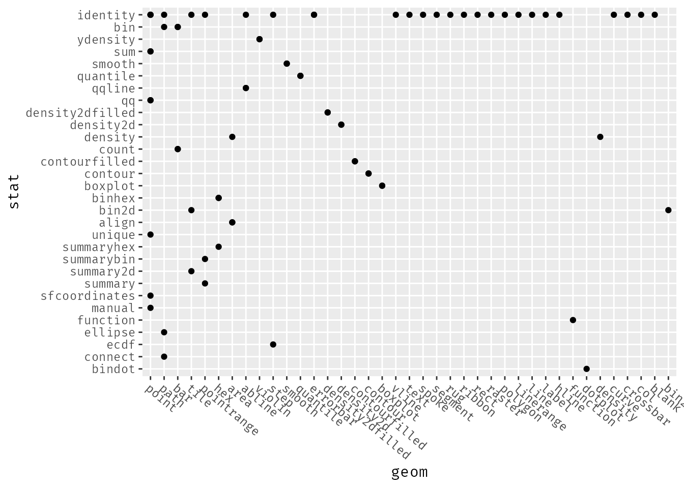
We can see that the most common stat by far is the identity stat. What’s that about?
The identity stat is a stat that does nothing.2 It takes the data as-is and passes it to the geom’s aesthetics.
Geoms that use the identity stat can be thought of a the most basic building blocks of {ggplot2} - many types of lines, bars/tiles, points, areas, etc. These are the geoms you’d probably use with annotate().3 We can see such geoms are often used with other stats as well:
ggdata |>
  filter("StatIdentity" %in% stat, .by = geom) |>
  mutate(
    stat = str_remove(stat, "Stat") |> str_to_lower(),
    geom = str_remove(geom, "Geom") |> str_to_lower(),

    is_identity = if_else(stat == "identity", "identity", "other"),
    geom = fct_reorder(factor(geom), geom, .fun = length)
  ) |>
  ggplot(aes(stat, geom, fill = geom)) +
  facet_grid(cols = vars(is_identity), scales = "free_x", space = "free_x") +
  geom_point(
    shape = 21,
    color = "black",
    size = 3
  ) +
  ggrepel::geom_label_repel(
    aes(label = ggfunction),
    family = "fira code",
    layout = 2,
    force = 10,
    max.overlaps = Inf
  ) +
  theme(
    title = element_text(family = "fira code"),
    axis.text = element_text(family = "fira code")
  ) +
  scale_fill_viridis_d(option = "A", end = 1, begin = 0.2) +
  scale_x_discrete(guide = guide_axis(angle = -40)) +
  guides(fill = "none")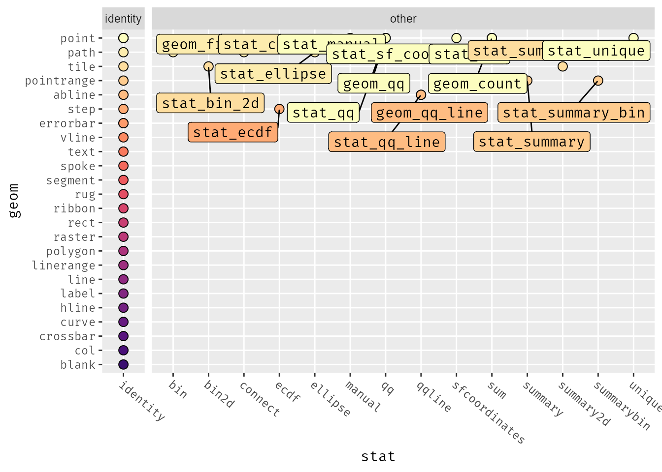
For example, the point geom is used by {ggplot2} together with 7 other non-identity stats.
{ggplot2} provides many stats that basically can only be used with a specific geom (and vice versa). These geom-stat pairs are almost exclusive to one another - think of a boxplot for example, which is a unique geom that has little meaning without the boxplot stat.
p2 <- ggplot(mpg, aes(class, hwy)) +
  geom_boxplot()
p2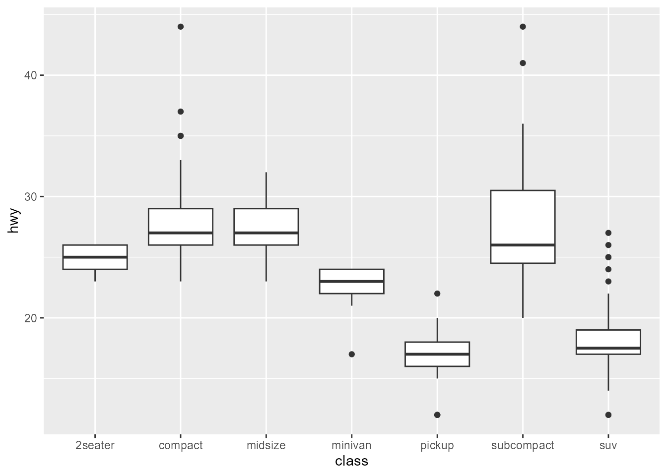
layer_data(p2, i = 1) |>
  # see computed variables:
  select(x, ymin:ymax, width, outliers)
#>   x ymin lower middle upper ymax width                       outliers
#> 1 1   23  24.0   25.0  26.0   26   0.9
#> 2 2   23  26.0   27.0  29.0   33   0.9                 35, 37, 35, 44
#> 3 3   23  26.0   27.0  29.0   32   0.9
#> 4 4   21  22.0   23.0  24.0   24   0.9                             17
#> 5 5   15  16.0   17.0  18.0   20   0.9                 12, 12, 12, 22
#> 6 6   20  24.5   26.0  30.5   36   0.9                         44, 41
#> 7 7   14  17.0   17.5  19.0   22   0.9 12, 12, 25, 24, 27, 25, 26, 23
The table below lists all the geom-stat pairs in {ggplot2}:
ggdata_pairs <- ggdata |>
  filter(
    stat != "StatIdentity",
    !help_page %in%
      c(
        "geom_abline",
        "geom_linerange",
        "ggsf",
        "stat_summary",
        "stat_summary_2d"
      ),
    !ggfunction %in% c("geom_col", "geom_freqpoly"),
    !str_detect(ggfunction, "(bin2d|density2d|binhex)")
  ) |>
  filter(n() > 1, .by = c(help_page)) |>
  arrange(help_page) |>
  mutate(
    stat = str_remove(stat, "Stat") |> str_to_lower(),
    geom = str_remove(geom, "Geom") |> str_to_lower()
  )

ggdata_pairs |>
  pivot_wider(
    names_from = type,
    values_from = ggfunction,
    id_cols = c(help_page, geom, stat),
    names_prefix = "type_"
  ) |>
  group_by(help_page) |>
  fill(starts_with("type_"), .direction = "downup") |>
  ungroup() |>
  distinct(help_page, type_geom, type_stat, .keep_all = TRUE) |>
  mutate(
    help_page = case_when(n() > 1 ~ help_page, .default = "Other topics"),
    .by = help_page
  ) |>
  gt(groupname_col = "help_page") |>
  cols_merge(
    columns = c(type_geom, stat),
    pattern = '{1}(stat = "{2}")'
  ) |>
  cols_merge(
    columns = c(type_stat, geom),
    pattern = '{1}(geom = "{2}")'
  ) |>
  opt_table_font(font = google_font("Fira Code")) |>
  tab_style(
    style = list(
      cell_text(weight = "bold")
    ),
    locations = cells_column_labels()
  ) |>
  tab_style(
    style = list(
      cell_text(weight = "bold")
    ),
    locations = cells_row_groups()
  ) |>
  cols_label(
    "type_geom" = "geom_",
    "type_stat" = "stat_",
    "help_page" = "Topic"
)| geom_ | stat_ |
|---|---|
| Other topics | |
| geom_bar(stat = "count") | stat_count(geom = "bar") |
| geom_bin_2d(stat = "bin2d") | stat_bin_2d(geom = "bin2d") |
| geom_boxplot(stat = "boxplot") | stat_boxplot(geom = "boxplot") |
| geom_count(stat = "sum") | stat_sum(geom = "point") |
| geom_density(stat = "density") | stat_density(geom = "density") |
| geom_hex(stat = "binhex") | stat_bin_hex(geom = "hex") |
| geom_histogram(stat = "bin") | stat_bin(geom = "bar") |
| geom_quantile(stat = "quantile") | stat_quantile(geom = "quantile") |
| geom_area(stat = "align") | stat_align(geom = "area") |
| geom_smooth(stat = "smooth") | stat_smooth(geom = "smooth") |
| geom_violin(stat = "ydensity") | stat_ydensity(geom = "violin") |
| geom_contour | |
| geom_contour(stat = "contour") | stat_contour(geom = "contour") |
| geom_contour_filled(stat = "contourfilled") | stat_contour_filled(geom = "contourfilled") |
| geom_density_2d | |
| geom_density_2d(stat = "density2d") | stat_density_2d(geom = "density2d") |
| geom_density_2d_filled(stat = "density2dfilled") | stat_density_2d_filled(geom = "density2dfilled") |
| geom_qq | |
| geom_qq(stat = "qq") | stat_qq(geom = "point") |
| geom_qq_line(stat = "qqline") | stat_qq_line(geom = "abline") |
When using the default geom= and stat= arguments, these pairs are interchangeable - meaning you can swap the stat_ function for the geom_ function from the table above. For example:
# g1 <- ggplot(mpg, aes(class))
# g1 + geom_bar() + g1 + stat_count()

# g2 <- ggplot(diamonds, aes(x, y)) + xlim(4, 10) + ylim(4, 10)
# g2 + geom_bin_2d() + g2 + stat_bin_2d()

# g3 <- ggplot(mpg, aes(class, hwy))
# g3 + geom_boxplot() + g3 + stat_boxplot()

# g4 <- ggplot(faithfuld, aes(waiting, eruptions, z = density))
# g4 + geom_contour() + g4 + stat_contour()
# g4 + geom_contour_filled() + g4 + stat_contour_filled()

# g5 <- ggplot(mpg, aes(cty, hwy))
# g5 + geom_count() + g5 + stat_sum()

# g7 <- ggplot(faithful, aes(x = eruptions, y = waiting))
# g7 + geom_density_2d() + g7 + stat_density_2d()
# g7 + geom_density_2d_filled() + g7 + stat_density_2d_filled()

# g8 <- ggplot(diamonds, aes(carat, price))
# g8 + geom_hex() + g8 + stat_bin_hex()

# g9 <- ggplot(diamonds, aes(carat))
# g9 + geom_histogram() + g9 + stat_bin()

# df <- data.frame(y = rt(200, df = 5))
# g10 <- ggplot(df, aes(sample = y))
# g10 + stat_qq() + stat_qq_line() + g10 + geom_qq() + geom_qq_line()

# g11 <- ggplot(mpg, aes(displ, 1 / hwy))
# g11 + geom_quantile() + g11 + stat_quantile()

# huron <- data.frame(year = 1875:1972, level = as.vector(LakeHuron))
# g12 <- ggplot(huron, aes(year, level))
# g12 + geom_area() + g12 + stat_align()

# g13 <- ggplot(mpg, aes(displ, hwy))
# g13 + geom_smooth() + g13 + stat_smooth()

g14 <- ggplot(mtcars, aes(factor(cyl), mpg))
(g14 + geom_violin() + ggtitle("geom_violin()")) +
  (g14 + stat_ydensity() + ggtitle("stat_ydensity()")) &
  theme(plot.title = element_text(family = "fira code"))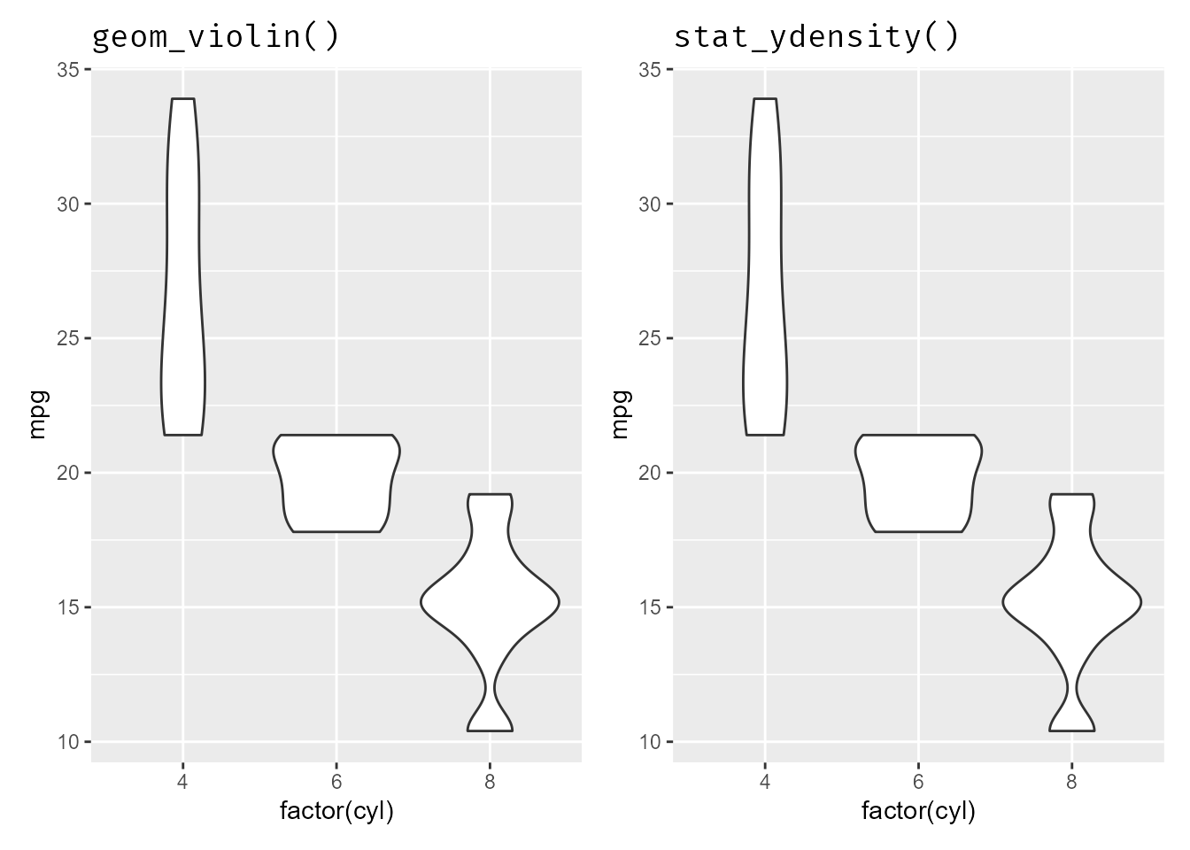
The only exception is geom/stat_density() for some reason?
g6 <- ggplot(diamonds, aes(carat))
(g6 + geom_density() +
    labs(title = "geom_density()",
         subtitle = 'stat = "density", geom = "area"')) +
  (g6 + stat_density() +
     labs(title = "stat_density()",
          subtitle = 'stat = "density", geom = "ribbon"')) &
  theme(plot.title = element_text(family = "fira code"),
        plot.subtitle = element_text(family = "fira code"))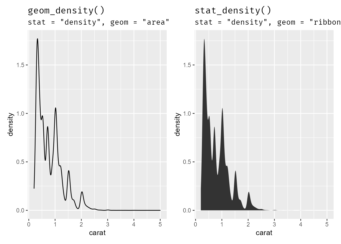
Understanding the relationship between geoms and stats is a key part of mastering {ggplot2}. Building a mental model of how {ggplot2} processes your data – really understanding its underlying grammar – allows you to move away from simply using defaults to confidently customizing your plots. When you understand that a function like geom_bar() is just a shortcut for layer(stat = "count", geom = "bar"), you can start to think about how you might pair different geoms with existing stats, or how to use the different computed variables provided by a stat.
Personally I’m looking forward to experimenting with the new stat_manual()!
So the next time you create a plot, I encourage you to use layer_data() and ask not what the data can do for you, but what you can do to your data!