# For plotting
library(ggplot2)

# For extracting SDT parameters
library(neuropsychology)I recently came across a paper that explained the equality between the parameters of signal detection theory (SDT) and the parameters of logistic regression in which the state (“absent”/“present”) is used to predict the response (“yes”/“no”, but also applicable in scale-rating designs) (DeCarlo, 1998).
Here is a short simulation-proof for this equality.
Setup
For this simulations we will need the following packages:
We will also need to make sure, for the logistic regression analysis, that our factors’ dummy coding is set to effects-coding - otherwise the intercept’s meaning will not correspond to the criterion (aka the overall response bias):
options(contrasts = c('contr.sum', 'contr.poly'))The Simulations
n <- 100L
B <- 100L
We’ll run 100 simulations with 100 trials each.
Simulation Code
set.seed(1)

SDT_params <- function(state,resp) {
  tab <- table(state,resp)

  sdt_res <- dprime(
    n_hit  = tab[2,2],
    n_miss = tab[2,1],
    n_fa   = tab[1,2],
    n_cr   = tab[1,1]
  )

  c(sdt_res$dprime , sdt_res$c)
}

logistic_reg_params <- function(state,resp){
  fit <- glm(resp ~ state, family = binomial())

  coef(fit)
}

# initialize
res <- data.frame(d_    = numeric(B),
                  c_    = numeric(B),
                  int   = numeric(B),
                  slope = numeric(B))

# Loop
for (b in seq_len(B)) {
  true_sensitivity <- rexp(1,10) # random
  true_criterion <- runif(1,-1,1) # random

  # true state vector
  state_i <- rep(c(F,T), each = n/2)

  # response vector
  Xn <- rnorm(n/2) # noise dist
  Xs <- rnorm(n/2, mean = true_sensitivity) # signal + noise dist
  X <- c(Xn,Xs)
  resp_i <- X > true_criterion

  # SDT params
  res[b,1:2] <- SDT_params(state_i,resp_i)

  # logistic regression params
  res[b,3:4] <- logistic_reg_params(state_i,resp_i)
}
Results
SDT parameters are on a standardized normal scale, meaning they are scaled to \(\sigma=1\). However, the logistic distribution’s scale is \(\sigma=\pi/\sqrt3\). Thus, to convert the logistic regression’s parameters to the SDT’s we need to scale both the intercept and the slope by \(\sqrt3/\pi\) to have them on the same scale as \(c\) and \(d'\).1 Additionally,
- The slope must be also scaled by \(-2\) due to R’s default effects coding.
- The intercept must also be scaled by \(-1\) - see paper for the full rationale.
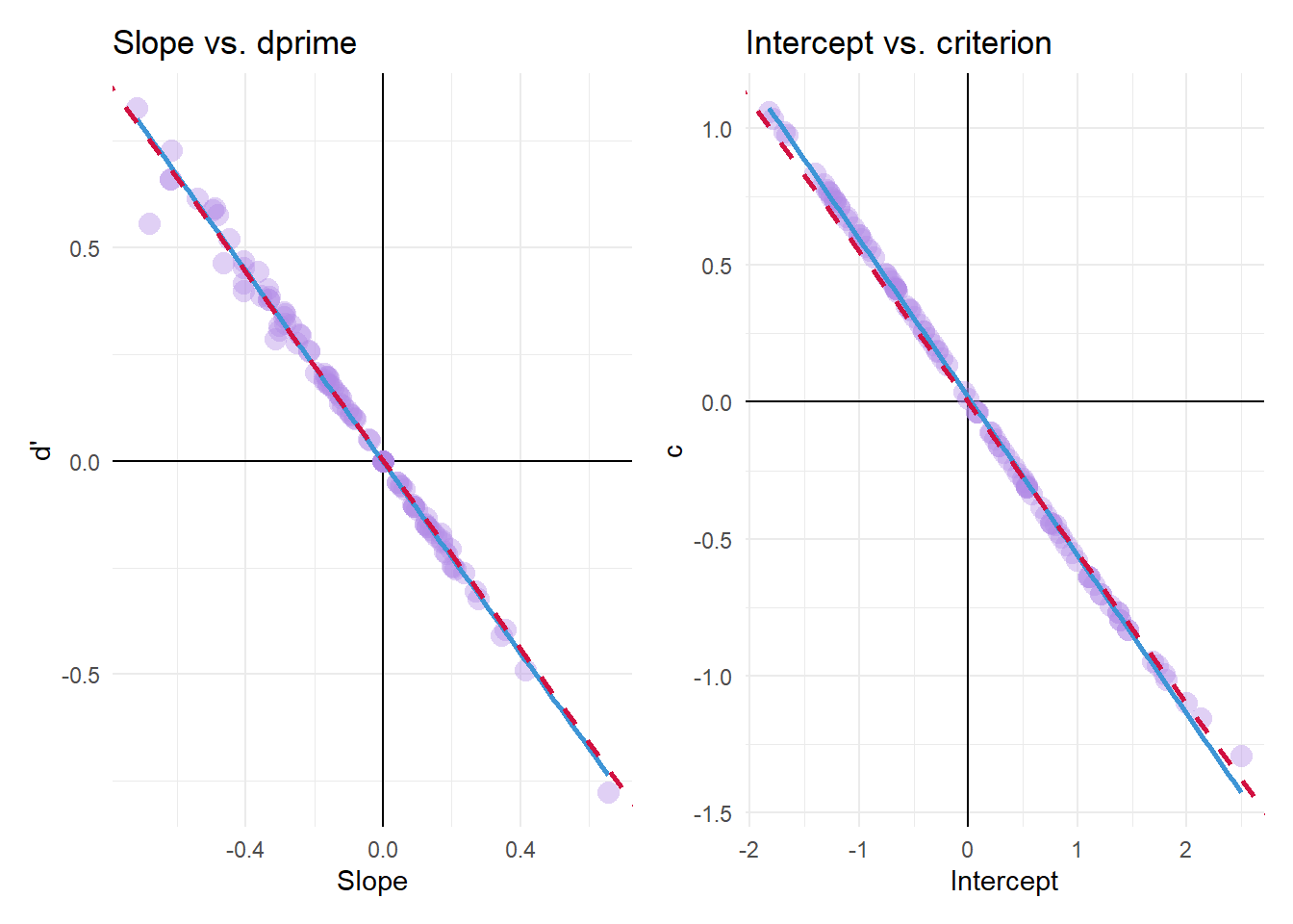
The red-dashed line represents the expected regression line predicting the SDT parameters from their logistic counterparts:
- \(d' = -2\times\frac{\sqrt{3}}{\pi}\times Slope\)
- \(c = -\frac{\sqrt{3}}{\pi}\times Intercept\)
(The blue line is the empirical regression line.)
Conclusions
It is also possible to extend this equality to multi-level designs with generalized linear mixed models (GLMM; see chapters 3 and 9 in Modeling Psychophysical Data in R)2, but I see no reason this wouldn’t be possible… One could model random effects per subject, and the moderating effect of some \(X\) on sensitivity could in theory be modeled by including an interaction between \(X\) and state; similarly, the moderating effect of \(X\) on the criterion can be modeled by including a main effect for \(X\) (moderation the intercept).